The idea: count the grey levels, then remap them
A grey image is a grid of numbers. Here it is 8×8 = 64 pixels, and each pixel has one of L = 8 grey levels: 0 is black, 7 is white. The histogram counts how many pixels have each level. A dull, low-contrast image uses only a few levels next to each other. Histogram equalization builds a new level for each old level from the running sum of those counts, so the pixels spread out over the whole range from 0 to 7.
Pick a transform to run it on the image, step by step. The top row shows the input image, the mapping curve and the output image. The bottom row shows the two histograms and the mapping table between them. Output → Input feeds the result back in, so you can transform it again.
A histogram of a small image
The histogram is a list of L counts n0 … n7. They always add up to the number of pixels, 64. Divided by 64 they are the fraction of the image at each level, a discrete probability distribution. The histogram says nothing about where the pixels are, only how many there are of each level.
| image | counts n0 … n7 | levels used | mean, sd |
|---|---|---|---|
| low contrast | 0 0 8 20 24 12 0 0 | 2–5 | 3.63, 0.93 |
| dark | 4 20 26 8 4 2 0 0 | 0–5 | 1.91, 1.10 |
| washed out | 0 0 2 4 8 26 20 4 | 2–7 | 5.09, 1.10 |
The standard deviation (sd) of the levels is a simple measure of contrast: small means most pixels look alike.
Point transforms: one table for every pixel
A point transform s = T(r) computes each new pixel from the old pixel's own level r, nothing else. With 8 levels, T is just a table of 8 numbers, a lookup table. All pixels of one level look up the same entry, so they move together: one histogram bar moves to a new place as a whole. Two bars can land on the same level and merge, but one bar can never split.
Filters that look at the neighbours of a pixel (blur, sharpen, edges) are not point transforms. See Convolution for those.
Equalization: the running sum is the mapping
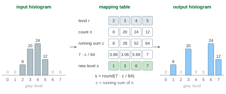
Equalization wants every level to hold about the same number of pixels. It walks the levels from dark to light and keeps a running sum ck = n0 + … + nk: the number of pixels at level k or darker. Then it scales that to the level range and rounds:
s_k = round( (L − 1) · c_k / N ) = round( 7 · c_k / 64 )
The running sum divided by N is the cumulative distribution function (CDF) of the levels; see PDF vs CDF. Where the histogram is tall, the sum jumps, so those levels get pushed far apart. Where it is empty, the sum stays flat, and no output level is wasted there. On the low-contrast image (Demo 1: equalize a low-contrast image):
| level r | 2 | 3 | 4 | 5 |
|---|---|---|---|---|
| count n | 8 | 20 | 24 | 12 |
| running sum c | 8 | 28 | 52 | 64 |
| 7 · c / 64 | 0.88 | 3.06 | 5.69 | 7 |
| new level s | 1 | 3 | 6 | 7 |
The levels now run from 1 to 7 instead of 2 to 5, and the sd grows from 0.93 to 2.06. The table is the whole method: it costs one pass to count, eight additions, and one lookup per pixel.
Why the result is not flat
A perfectly flat histogram would have 8 pixels at every level. That cannot happen here: the 24 pixels at level 4 all go to the same new level, so that bar stays 24 tall. With few levels, equalization only spreads the bars; it cannot cut them. On the dark image, levels 4 and 5 both map to 7 and merge: 6 levels in, 5 levels out (Demo 4: a dark image, two levels merge).
Equalizing an equalized image changes nothing. The output's running sum already rises in even steps, so every used level maps to itself (Demo 3: equalizing twice changes nothing).
Stretching, gamma and log
The other transforms use a fixed formula. They do not look at the counts (stretching only reads the darkest and the lightest level).
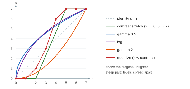
| transform | s = T(r) | table for r = 0 … 7 | good for |
|---|---|---|---|
| contrast stretching | (r − rmin) · 7 / (rmax − rmin) | 0 0 0 2 5 7 7 7 (low contrast) | a narrow range, used evenly |
| gamma 0.5 | 7 · (r/7)0.5 | 0 3 4 5 5 6 6 7 | dark images: lifts the shadows |
| log | 7 · ln(1 + r) / ln 8 | 0 2 4 5 5 6 7 7 | a huge range, such as a Fourier spectrum |
| gamma 2 | 7 · (r/7)2 | 0 0 1 1 2 4 5 7 | washed-out images: darkens the bright end |
| negative | 7 − r | 7 6 5 4 3 2 1 0 | looking at dark detail, film negatives |
Every value is rounded and kept in 0…7. On the dark image, gamma 0.5 sends levels 1, 2, 3 to 3, 4, 5 (Demo 5: gamma 0.5 lifts the shadows); log sends them to 2, 4, 5 (Demo 6: log transform on the dark image). Gamma 2 does the opposite on the washed-out image: levels 5 and 6, which hold 46 of the 64 pixels, go to 4 and 5 (Demo 7: gamma 2 on a washed-out image). Screens and cameras use gamma curves too, around γ = 2.2, to match how eyes see brightness.
Equalization vs stretching
On the low-contrast image both use the full range 0–7 or close to it, but they place the bars differently (Demo 2: contrast stretching on the same image):
| contrast stretching | histogram equalization | |
|---|---|---|
| mapping for 2, 3, 4, 5 | 0, 2, 5, 7 | 1, 3, 6, 7 |
| built from | the darkest and lightest level only | every count (the CDF) |
| shape | a straight line: equal gaps | steep where the histogram is tall |
| mean, sd after | 3.81, 2.30 | 4.63, 2.06 |
| one stray pixel at 0 and one at 7 | does nothing (range is already 0–7) | barely changes the result |
Stretching is predictable and keeps the look of the image. Equalization adapts to the image, which helps on pictures with a few crowded levels but can make noise and flat areas look harsh.
See also Sampling and Aliasing for how a picture becomes pixels in the first place, and JPEG and the DCT for how grey levels are stored compactly.
See also Morphology: Erosion and Dilation, which cleans up a thresholded binary image by removing noise specks and filling holes.
See also Thresholding and Otsu's Method, which cuts the histogram into two classes instead of spreading it out.
What the page leaves out
Real images have 256 levels (8 bits) and millions of pixels, so the bars are thin and equalization comes out much flatter. Colour images are usually equalized on the brightness channel only. Common variants: the form s = round((c − cmin) · (L − 1) / (N − cmin)), which sends the darkest used level to 0; adaptive equalization (AHE, CLAHE), which uses a histogram per tile and clips tall bars; and histogram matching to a target shape. Piecewise-linear stretching, bit-plane slicing, thresholding, and filters that use neighbours (smoothing, sharpening, edge detection) are left to other pages.