The idea: one cell, used again at every step
Text, speech and sensor readings come as sequences. A recurrent neural network (RNN) reads them one token at a time with the same cell and the same weights at every step. The only thing it carries from one step to the next is a vector called the hidden state h. Drawn step by step, the loop becomes a chain: the network unrolled over time.
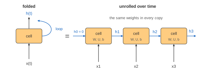
On this page the hidden state is a single number so every value fits on the canvas, and the weights are set by hand, as if already trained. Tokens come from a tiny vocabulary:
| token | x = (content, store, reset, query) | meaning |
|---|---|---|
| A | (1, 1, 0, 0) | a value +1 to remember |
| B | (−1, 1, 0, 0) | a value −1 to remember |
| · | (0, 0, 0, 0) | filler |
| R | (0, 0, 1, 0) | reset: forget the memory |
| ? | (0, 0, 0, 1) | query: read the memory out |
The RNN step
ht = tanh(W·xt + U·ht−1 + b), starting from h0 = 0. Here W = (2, 0, 0, 0),
U = 0.8 and b = 0. W reads the token, U reads the old state, and tanh squashes the sum into (−1, 1).
On A · B · · the state goes 0.964, 0.648, −0.902, −0.618, −0.458: the A fades and B overwrites it.
(Demo 1: RNN over 5 steps) With a real hidden vector, W and U are matrices and tanh is applied to each entry.
Backpropagation through time
Unrolled, the RNN is an ordinary deep network, so it is trained with backpropagation run backward along the chain: backpropagation through time (BPTT). The gradients from every step are summed into the one shared W, U and b. The page shows the factor that decides whether learning can reach far back: δt = ∂hT/∂ht, how much the last state depends on the state at step t.
By the chain rule δt = δt+1 · U · (1 − ht+1²): one multiply per step, by the recurrent weight times the slope of tanh.
The vanishing gradient
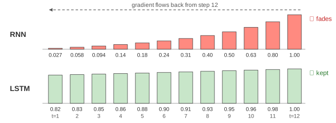
Each factor U·(1 − h²) is at most 0.8 here, so the product shrinks geometrically. On the 12-token sequence
A · · · · · · · · · · ? the gradient reaching step 1 is 0.027; over 50 steps 0.850
alone is 1.4·10−5. The error at the end cannot tell the early weights anything, so a plain RNN learns
short-range patterns only. That is the vanishing gradient. (Demo 2)
If |U| is large instead, the factors are above 1 and the gradient explodes; the usual fix is gradient clipping (rescale the gradient when its norm is too big). Vanishing has no such quick fix: it needs a different cell.
The LSTM cell
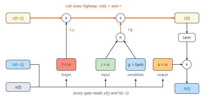
A long short-term memory cell (Hochreiter & Schmidhuber, 1997) keeps a second state, the cell state c, and three gates. A gate is a sigmoid, a number between 0 (closed) and 1 (open), that multiplies something:
| part | formula | on this page | job |
|---|---|---|---|
| forget gate f | σ(Wf·x + Uf·h + bf) | σ(4 − 8·store − 8·reset) | how much of the old c to keep |
| input gate i | σ(Wi·x + Ui·h + bi) | σ(8·store − 4) | how much of the candidate to write |
| candidate g | tanh(Wg·x + Ug·h + bg) | tanh(2·content) | the new value, in (−1, 1) |
| output gate o | σ(Wo·x + Uo·h + bo) | σ(8·query − 1) | how much of the memory shows in h |
| cell state | ct = f·ct−1 + i·g | the memory | |
| hidden state | ht = o·tanh(ct) | the output, and input to the next step |
The page's U weights inside the gates are 0, so each gate depends only on the token; a trained LSTM also looks at ht−1. On a filler token the forget gate is σ(4) = 0.982, the input gate σ(−4) = 0.018 and the output gate σ(−1) = 0.269: keep the memory, write nothing, show a little. (Demo 3: one step through the four gates)
Why the highway keeps memory and gradient
From one step to the next, c is multiplied by f and something is added. There is no tanh and no weight matrix on that path, so ∂ct/∂ct−1 = f (along the direct path). With f ≈ 1 the memory and the gradient both survive. After A, eleven forget gates of 0.982 leave c12 = 0.775, and the query token opens the output gate: h12 = 0.999 · tanh(0.775) = 0.649. (Demo 4)
| 12-token sequence A · · · · · · · · · · ? | RNN | LSTM | GRU |
|---|---|---|---|
| state at step 12 | h = 0.057 | c = 0.775, h = 0.649 | h = 0.906 |
| factor per step back | U·(1 − h²) ≤ 0.8 | f = 0.982 | (1 − z) + z·(1 − h̃²)·r ≈ 0.99 |
| gradient reaching step 1 | 0.027 | 0.819 | 0.900 |
(Demo 6: RNN vs LSTM on the same sequence; the GRU column is Demo 7.)
Forgetting on purpose
Keeping everything is not the goal. When the reset token R arrives the forget gate drops to σ(−4) = 0.018 and the cell
state falls from 0.897 to 0.016: the memory is wiped, and the gradient through that step is cut too. A store token does
the same before writing, so in A · · · B · · · the B overwrites A instead of adding to it.
(Demo 5) Early LSTMs had no forget gate; Gers et al. (2000) added it so a cell can reset itself.
Practitioners often start the forget-gate bias at 1 or more so that f begins near 1.
The GRU cell: two gates, no cell state
A GRU (gated recurrent unit, Cho et al. 2014) keeps the highway but drops the separate cell state: h itself is the memory. Pick model: GRU. Two gates instead of three:
| part | formula | on this page | job |
|---|---|---|---|
| update gate z | σ(Wz·x + Uz·h + bz) | σ(8·store + 8·reset − 4) | how much to replace: keep 1 − z of the old h, write z of the new |
| reset gate r | σ(Wr·x + Ur·h + br) | σ(4 − 8·store − 8·reset) | how much of the old h the candidate may see |
| candidate h̃ | tanh(W·x + U·(r·ht−1) + b) | tanh(2·content + r·h) | the new value |
| hidden state | ht = (1 − z)·ht−1 + z·h̃ | memory and output at once |
One update gate does the jobs of the LSTM's forget and input gates, tied together: what is kept and what is written add up to 1. There is no output gate, so the whole memory is always visible in h. On the filler tokens z = 0.018, so h shrinks only from 0.947 to 0.906 over 11 steps and the gradient reaching step 1 is 0.900 (Demo 7). At R both gates act: z = 0.982 replaces h, and r = 0.018 hides the old h from the candidate, so h drops from 0.935 to 0.033 (Demo 8). The GRU has about three quarters of the LSTM's parameters and usually works about as well. Libraries differ on the sign: PyTorch writes h = (1 − z)·h̃ + z·ht−1, so its z is the "keep" share.
Transformers
RNNs, LSTMs and GRUs all have to read a sequence one step at a time, which is slow to train on a GPU. Self-attention lets every token look at every earlier token directly, in parallel, so transformers replaced RNNs for most language tasks; see How a Large Language Model Works. The basic layer both build on is in Neural Network: the Forward Pass.
What the page leaves out
Hidden vectors and weight matrices (here everything is one number), training the weights (they are set by hand), the gradient paths through h and the gates (BPTT here follows only h for the RNN and only the c highway for the LSTM; for the GRU it is exact, because its gates read only the token), truncated BPTT, peephole connections, bidirectional and stacked RNNs, and sequence-to-sequence models.