The idea: let every edge pixel vote for the lines through it
An edge detector such as Canny marks the pixels where the brightness jumps. It does not say which of them form a straight line. The Hough transform answers that with a vote. Each edge pixel votes for every line that passes through it. A line that many pixels vote for is a line in the image. The votes are counted in a grid of possible lines, the accumulator.
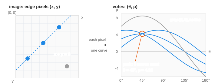
The page uses an 8 × 8 edge image so every vote is visible. Pixel (x, y) is column x, row y, both from 0, with y going down; the origin is the centre of pixel (0, 0), as in OpenCV. The accumulator has 12 columns for θ (15° apart) and 18 rows for ρ (1 pixel apart): 216 cells.
Writing a line as (θ, ρ)
The school form y = mx + b does not work well here. A vertical line has no slope m, and m can be any number, so the grid would have to be endless. Instead a line is written by its normal, the shortest arrow from the origin to the line:
ρ = x cos θ + y sin θ
θ  the angle of the normal, 0° ≤ θ < 180°
ρ  its signed length: the distance from the origin to the line
Every line has exactly one such pair, and both numbers stay in a small range: θ in half a turn, |ρ| at most the image diagonal. The row y = 2 is θ = 90°, ρ = 2. The column x = 5 is θ = 0°, ρ = 5. The diagonal x + y = 7 is θ = 45°, ρ = 7 / √2 = 4.95. When the line passes on the other side of the origin, ρ is negative. The pair is a polar coordinate of the foot of the normal; polar coordinates themselves are on Polar Coordinates.
One pixel, one curve
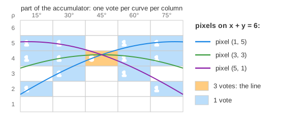
Fix a pixel (x, y) and turn θ. For each θ there is exactly one line through the pixel, with ρ = x cos θ + y sin θ. Plotted over θ this is a smooth wave, a sinusoid ρ = √(x² + y²) · cos(θ − φ). The grid only has 12 columns, so the pixel adds one vote per column, in the row ρ rounded to a whole number. Pixel (1, 5) votes in rows 1 2 3 4 5 5 5 5 4 3 2 0 for θ = 0°, 15°, …, 165° (Demo 1: one pixel votes along a curve). Every pixel gives 12 votes, so after n pixels the grid holds 12n votes.
Pixels on a line meet in one cell
All pixels on one line share that line's (θ, ρ). So their curves all pass through the same cell, and that cell gets one vote from each of them. Pixels (1, 5) and (5, 1) both lie on x + y = 6, and their curves cross in (45°, 4): the only cell with 2 votes (Demo 2). Eight pixels on x + y = 7 give cell (45°, 5) eight votes (Demo 3). The pixels do not have to touch: a dashed line or a line behind an object still collects its votes.
Finding the peaks
A cell counts as a line when it has at least min votes (OpenCV's threshold argument)
and is also the largest in its 3 × 3 block of neighbouring cells. The second rule matters because a strong line leaks votes
into the cells next to its peak: its pixels round to the same row in the neighbouring θ columns too. In the two-lines image
the row y = 2 gives (90°, 2) eight votes, and the cell next to it, (105°, 1), still gets 5. Without the 3 × 3 rule it would
be reported as a second, slanted line (Demo 4: two lines, two peaks). The diagonal x + y = 9 gives (45°, 6)
seven votes. Pixel (7, 2) lies on both lines and voted for both.
The line drawn back on the image uses the cell's centre, ρ = 6, while the pixels lie on ρ = 9 / √2 = 6.36. With a coarse grid the line found is close to the real one, not exactly on it.
Noise and false lines
Four extra noise pixels in the same image add 48 votes. Most land in cells with 1 to 3 votes: scattered, not piled up. The two real lines still stand out. But a few cells gather votes by chance, from noise pixels and line pixels that happen to be nearly in a row:
| min votes | lines found | what happens |
|---|---|---|
| 5 | 2 | (90°, 2) = 8 and (45°, 6) = 7, the real lines (Demo 5) |
| 4 | 4 | also (15°, 1) and (45°, 4) with 4 votes each: chance alignments of 2 noise pixels and 2 line pixels (Demo 6) |
So min votes is the shortest line you are willing to believe in, counted in pixels. Set it from the image size and the length of the lines you expect.
Bin size: precision against tolerance
The last image is a line at a slope of −1/2, drawn on pixels. A line drawn on pixels is a staircase, not exactly straight, and its normal (about 63.4°) falls between the 60° and 75° columns. So no cell gets all 8 votes: the best, (60°, 6), gets 5, and the cells (75°, 5) and (45°, 6) get 4 each. With min votes 6 the line would be missed (Demo 7: a line between two θ bins).
One cell is a strip in the image: all points whose ρ, for that θ, rounds to the cell's row. Cell (60°, 6) is the strip 5.5 ≤ ρ < 6.5, one pixel wide, and only 5 of the 8 staircase pixels fit in it.
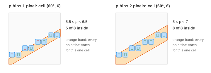
Finer θ steps alone do not help here: with 5° steps the best cell still has 5 votes, with 1° steps 6. Wider ρ bins
(2 pixels) put all 8 votes in one cell, even with 15° steps, but then two lines 2 pixels apart fall into one cell.
So the bin size is a trade-off between precision and tolerance for pixels that are not quite in a row. The cost
grows with it too: the grid has Nθ × Nρ cells, and voting costs one addition per edge pixel per
θ column. OpenCV's tutorial uses rho = 1 and theta = π/180 (180 columns) on whole photos.
Beyond straight lines
- Circles: a circle has three numbers (centre a, b and radius r), so the vote goes into a 3-D grid.
- Probabilistic Hough (OpenCV
HoughLinesP) votes with a random part of the pixels and returns line segments with end points instead of endless lines. - Any shape with a few parameters can be found the same way; the grid grows with each parameter.
Picking peaks in a grid of scores is like keeping the best box in non-maximum suppression for object detection: keep the local best, drop its near copies.
See also Harris Corner Detection, which finds corner points from the gradients instead of voting for lines.
What the page leaves out
Real edge images have thousands of edge pixels and grids of 180 × 1000 cells or more. How the edge pixels are found (blur, gradient, thresholds) is on the Canny page, and turning a grey image into black and white is Otsu thresholding. Not shown: voting only along the gradient direction (one vote per pixel instead of 12), weighting votes by edge strength, smoothing the accumulator, splitting a line into segments, the circle and generalized Hough transforms, and how OpenCV picks its peaks (it compares only the 4 side neighbours).