The idea: a window that changes in two directions
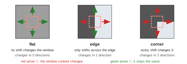
A corner is a good point to track from one photo to the next, because it can only match in one place. Put a small window on the image and slide it a little. On a flat area the window sees the same thing wherever it moves. On an edge it changes when it moves across the edge, but not when it moves along it. At a corner it changes whichever way it moves. Chris Harris and Mike Stephens (1988) turned this test into a few sums of gradients and one number per pixel, the response R.
The page works on a 10 × 10 image so every number fits on the screen. Pixel (x, y) means column x, row y, both counted from 0, with y going down. The default image is a bright rectangle (140) on a dark background (40), columns 2–7 and rows 2–6. The six panels are the image, the two gradients, the response R, the corners found and the structure matrix of one chosen pixel.
1. Gradients
The gradient says how fast the brightness changes at a pixel. The page uses the simplest kind, a central difference: Ix is the right neighbour minus the left one, halved; Iy is the pixel below minus the pixel above, halved. At the rectangle's top-left corner (2, 2) both are (140 − 40) ÷ 2 = 50. Along the left side Ix = 50 and Iy = 0; along the top Ix = 0 and Iy = 50; inside and outside both are 0. Real detectors often use the Sobel kernels instead, shown on Canny Edge Detection; how a kernel slides over an image is on Convolution in a CNN.
2. The structure matrix
One gradient is not enough. At a single pixel the matrix [Ix² IxIy; IxIy Iy²] always has determinant Ix²·Iy² − (Ix·Iy)² = 0: one arrow points in one direction only. A corner shows up when the gradients in a small neighbourhood point in different directions. So Harris adds them up over a window (here 3 × 3, all weights 1):
M = [ Sxx  Sxy ]    Sxx = ΣIx²   Syy = ΣIy²   Sxy = ΣIx·Iy
    [ Sxy  Syy ]    (sums over the 9 pixels of the window)
This structure matrix M describes how the window changes when it is shifted by a small step (u, v): the change is about u²·Sxx + 2uv·Sxy + v²·Syy. For the corner pixel (2, 2), 4 of the 9 window pixels have Ix = 50, 4 have Iy = 50 and one has both, so Sxx = 4 × 2500 = 10 000, Syy = 10 000 and Sxy = 2500 (Demo 4: a corner pixel).
3. Eigenvalues: flat, edge, corner
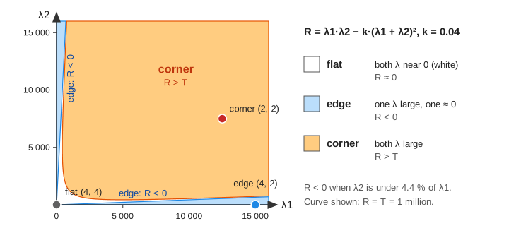
The two eigenvalues λ1 ≥ λ2 of M are how much the window changes in its most-changing and its least-changing direction (eigenvalues in general are on Eigenvectors). That gives the three cases directly:
| pixel of the rectangle | M | λ1, λ2 | R (million) | case |
|---|---|---|---|---|
| (4, 4) inside | all 0 | 0, 0 | 0 | flat (Demo 2) |
| (4, 2) top side | Syy = 15 000, rest 0 | 15 000, 0 | −9 | edge (Demo 3) |
| (2, 2) corner | 10 000, 10 000, Sxy 2500 | 12 500, 7 500 | 77.75 | corner (Demo 4) |
Eigenvalues do not care how the edge is turned. On the rotated square the slanted edge pixel (2, 2) has Sxx = Syy = Sxy = 12 500. Every entry is large, yet det(M) = 0, so λ2 = 0 and λ1 = 25 000: still an edge. The square's four tips are found as corners just like the rectangle's (Demo 6: rotated square).
4. The response R
Computing eigenvalues takes a square root per pixel, which was slow in 1988. Harris used two facts instead: det(M) = λ1·λ2 and trace(M) = λ1 + λ2. Then
R = det(M) − k·trace(M)² = λ1·λ2 − k·(λ1 + λ2)² k = 0.04- Both λ large: the product wins, R is large and positive. Corner (2, 2): 93 750 000 − 0.04 × 20 000² = 77 750 000.
- One λ large, the other near 0: the product is near 0, R is negative. Edge (4, 2): 0 − 0.04 × 15 000² = −9 000 000.
- Both near 0: R is near 0. Flat.
With k = 0.04, R is below 0 exactly when λ2 is less than about 4.4 % of λ1. The R panel shows R in millions: orange blobs at the four corners, blue bands along the sides. On the straight edge every R is 0 or negative, so no pixel can ever be a corner (Demo 5: straight edge).
5. Threshold and non-maximum suppression
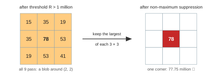
A corner is not one pixel in R. Every pixel whose 3 × 3 window holds part of the corner gets a large R, so the threshold R > 1 million keeps 36 pixels on the rectangle: four blobs of 9. Non-maximum suppression keeps a pixel only if its R is the largest in its own 3 × 3 neighbourhood (on a tie, the first one in reading order). Each blob shrinks to one pixel, and the 36 become the 4 corners (2, 2), (7, 2), (2, 6), (7, 6) (Demo 1). The same idea, applied to boxes instead of pixels, is on Object Detection.
Harris finds inside corners too. The L shape has five outside corners and one inside corner; the inside one is found at the dark pixel (5, 4) next to it, with the same R = 77.75 million but Sxy = −2500, because there the two slopes go in opposite ways (Demo 7: L shape).
The threshold depends on the contrast. Every gradient is proportional to the contrast, M to its square and R to its 4th power. The faint rectangle has contrast 40 instead of 100, so its corners have R = 77.75 × 0.4⁴ = 1.99 million. They pass R > 1 million but not R > 10 million, which finds 0 corners (Demo 8: faint rectangle, high threshold). That is why tools often use a threshold relative to the largest R, such as 1 % of it in the OpenCV tutorial.
Choosing k, the window and the threshold
- k is usually 0.04 to 0.06. A larger k pushes R down, so fewer pixels count as corners and more as edges.
- The window sets the scale. Two corners closer than the window merge into one blob and one answer; a larger window finds larger corners and ignores small ones.
- The threshold trades missed corners against noise. Too high loses faint corners; too low keeps noise as false corners.
Lines and circles are found differently: by voting, on Hough Transform.
What the page leaves out
Real detectors weight the window with a Gaussian (σ about 1–2) instead of a 3 × 3 box, often blur the image and
use Sobel derivatives first, and work on images thousands of pixels wide. OpenCV's cornerHarris takes
the window size, the Sobel size and k; its border handling and scaling differ from this page. Shi and Tomasi
replaced R by min(λ1, λ2) (goodFeaturesToTrack). Not shown: corners found at several scales
(Harris–Laplace), sub-pixel corner positions, colour images, faster detectors such as FAST, and the descriptors
(SIFT, ORB) that describe the patch around each corner so two photos can be matched.
On the mind map
References
Chris Harris and Mike Stephens — A Combined Corner and Edge Detector, Alvey Vision Conference (1988)
OpenCV — Harris Corner Detection tutorial
OpenCV — cornerHarris and goodFeaturesToTrack reference
Richard Szeliski — Computer Vision: Algorithms and Applications, chapter on feature detection