The idea: a density and its running total
A random variable X can be described two ways. The probability density function (PDF) f(x) says where the values are crowded. The cumulative distribution function (CDF) F(x) = P(X ≤ x) says how much probability lies at or left of x. The link between them is one sentence: the area under the PDF left of x is the height of the CDF at x.
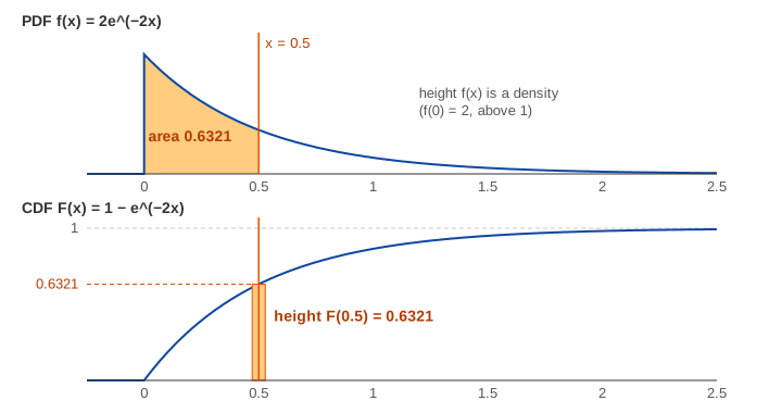
The canvas draws the PDF on top and the CDF below on the same x axis, so a vertical line at x passes through both. Demo: area under the PDF = height of the CDF shades the area, turns it into one number and carries it down.
A density is not a probability
For a continuous X the chance of any single value is 0: P(X = 0.5) = 0. Only intervals have probability, and that probability is an area: P(a < X ≤ b) = ∫ab f(x) dx. The height f(x) is probability per unit of x, so it can be larger than 1. For the exponential with rate 2, f(0) = 2. What must hold is f(x) ≥ 0 and a total area of 1.
The CDF is the area so far
F(x) = P(X ≤ x) = ∫ f(t) dt from −∞ to xSo F starts at 0 on the far left, ends at 1 on the far right and never goes down. It climbs fast where the density is tall and is flat where the density is 0 (Demo: sweep x, the CDF grows). For a uniform density the area grows at a constant rate, so the CDF is a straight line, F(x) = x/4 on [0, 4] (Demo: uniform, a straight-line CDF).
Probabilities of intervals: F(b) − F(a)
The area between a and b is the area left of b minus the area left of a. On the CDF that is a difference of two heights. For N(0, 1): P(−1 < X ≤ 1) = Φ(1) − Φ(−1) = 0.8413 − 0.1587 = 0.6827, the "68%" of the 68–95–99.7 rule (Demo: P(a < X ≤ b) = F(b) − F(a)). The green area on the PDF and the green part of the bar on the CDF are the same number.
The slope of the CDF is the PDF
Moving x a little, by dx, adds a thin strip of area about f(x)·dx. So the CDF rises at rate f(x): F′(x) = f(x). The tangent to the CDF at x = 0.5 for rate 2 has slope 2e−1 = 0.7358, the height of the density there; at 0 the slope is 2 (Demo: slope of the CDF is the PDF). Going one way you integrate (PDF → CDF), the other way you differentiate (CDF → PDF).
Discrete variables: PMF bars and a staircase
A discrete X, such as the sum of two dice, has a probability mass function (PMF) p(k) = P(X = k): bars whose heights are probabilities and add up to 1. Its CDF adds the bars up, so it is a staircase: flat between the values and jumping by p(k) at each k. F(7) = (1 + 2 + 3 + 4 + 5 + 6)/36 = 21/36 = 0.5833.
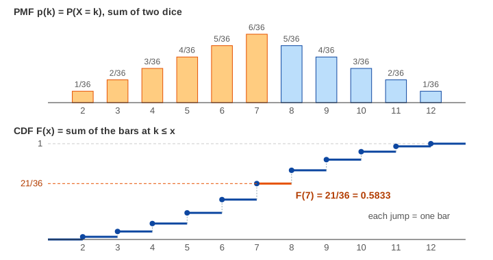
Here < and ≤ are different: P(6 < X ≤ 8) = F(8) − F(6) = 26/36 − 15/36 = 11/36 = 0.3056 counts 7 and 8 but not 6 (Demo: two dice, PMF bars and a staircase CDF). For a continuous X the endpoints carry no probability, so it does not matter.
Reading the CDF backwards: quantiles
The quantile for p is the x where F(x) = p, written F−1(p). Start at height p, go across to the curve and down. The median is F−1(0.5): for rate 2 that is ln 2 / 2 = 0.3466, below the mean 0.5 because the long right tail pulls the mean up (Demo: median from the CDF). p-values in hypothesis tests and z tables are CDF readings too.
PMF vs PDF vs CDF
| PMF p(k) | PDF f(x) | CDF F(x) | |
|---|---|---|---|
| for | discrete X | continuous X | both |
| height means | P(X = k) | probability per unit of x | P(X ≤ x) |
| range | 0 … 1 | 0 … ∞ (can exceed 1) | 0 … 1, never decreasing |
| total | bars add to 1 | area is 1 | F(∞) = 1 |
| P(a < X ≤ b) | add bars a < k ≤ b | area from a to b | F(b) − F(a) |
See also Binomial vs Poisson for two PMFs side by side, and the central limit theorem for histograms that turn into a density.
What the page leaves out
- Mixed distributions with both jumps and a density part, and the general measure-theory definition.
- The survival function 1 − F(x) and the hazard rate.
- Joint and conditional densities of two or more variables.
- Empirical CDFs from data and the Kolmogorov–Smirnov test.
- Sampling by inverse transform (X = F−1(U) for uniform U).