The idea: two ways to mix image patches
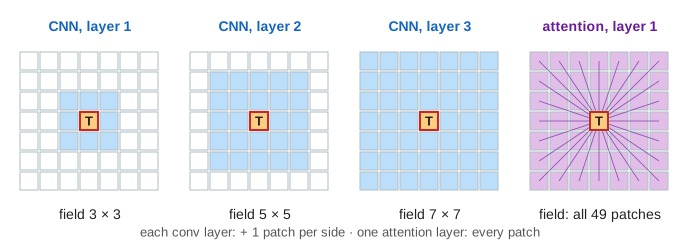
Both networks cut the image into a grid of small patches and, layer by layer, let each patch take in information from other patches. They differ in which patches. A convolutional network (CNN) mixes each patch with its 8 neighbours only. A vision transformer (ViT) uses self-attention: each patch looks at every patch of the image. The page runs both on the same image, one layer per Step, and asks one question: when has the target patch T seen all the patches it needs (the ? patches)?
CNN: a 3×3 window, stacked
A convolution layer slides a small kernel, here 3×3, over the grid. The new value of a patch is a weighted sum of the 3×3 window around it, with the same weights everywhere (see Convolution in a CNN). After one layer, T knows a 3×3 square; the next layer mixes windows that already hold 3×3 squares, so T knows 5×5. After L layers T's receptive field is (2L + 1) × (2L + 1) patches: it grows by one patch per side per layer. In the blue lane the field is tinted, and each ? turns into ✓ when it is inside.
For a local pattern this is perfect. An edge between T and its right neighbour is inside T's first 3×3 window, and the page's edge kernel (right column minus left column) gives +3 right away. (Demo: local edge, 16 × 16) But two objects in opposite corners of a 16 × 16 image are 8 patches from the middle patch, so the CNN needs 8 layers before any patch has seen both. (Demo: far corners, 16 × 16)
Vision transformer: every patch, one layer
A ViT turns each patch into a vector (a token) and runs the same attention as a language model. Each patch makes a query, a key and a value. T's query is compared with the key of every patch (a dot product, the score); softmax turns the N scores into weights that add up to 1, and T's new vector is the weighted sum of all N values. The page's head looks for object patches: an object gets score 3, background 0. On the edge image (48 object patches out of 256) each object patch gets weight 0.0171 and each background patch 0.0009, so T's output is 0.823. Any patch, near or far, is one hop away: both corners are reached in layer 1.
What it costs: weights and multiply-adds
Every patch carries C numbers (channels; the page uses C = 32). A 3×3 convolution from C to C channels has 9·C² weights and does 9·C² multiply-adds per patch. An attention layer has 4·C² weights (the matrices WQ, WK, WV and the output WO), but it pays for the reach: 4·C² per patch for the projections, plus N·C for the scores and N·C for the weighted sum. Per layer, for N patches:
| 3×3 conv | self-attention | |
|---|---|---|
| weights | 9·C² = 9,216 | 4·C² = 4,096 |
| patch pairs mixed | 9·N | N² |
| multiply-adds | 9·N·C² | 4·N·C² + 2·N²·C |
| 8 × 8 = 64 patches | 589,824 | 524,288 |
| 16 × 16 = 256 patches | 2,359,296 | 5,242,880 |
The weights do not depend on the image size, but attention's N² term does. The two layers cost the same when 9·C² = 4·C² + 2·N·C, that is at N = 2.5·C = 80 patches. On the small 8 × 8 image attention is a little cheaper and has fewer weights (Demo: local edge, 8 × 8); on 16 × 16 one attention layer costs 2.2 times a conv layer and mixes 65,536 patch pairs against 2,304 (Demo: local edge, 16 × 16). For far-apart patches the CNN pays with depth instead: 8 conv layers are 18.9 million multiply-adds against 5.2 million for one attention layer.
The demos in numbers
| demo | CNN layers | CNN multiply-adds | attention layers | attention multiply-adds | cheaper |
|---|---|---|---|---|---|
| local edge, 16 × 16 | 1 | 2.36 M | 1 | 5.24 M | CNN |
| far corners, 16 × 16 | 8 | 18.87 M | 1 | 5.24 M | attention |
| far corners, 8 × 8 | 4 | 2.36 M | 1 | 0.52 M | attention |
| local edge, 8 × 8 | 1 | 0.59 M | 1 | 0.52 M | attention |
Shuffle the patches: attention can't tell
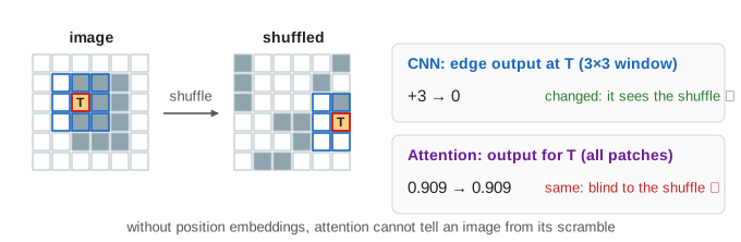
The attention score depends only on what is in the two patches, not on where they are. Shuffle the patches and every patch gets the same weights as before, just at other places, so T's output is exactly the same: 0.823 before and after. The network is permutation equivariant: it cannot tell the picture from a scrambled one. The conv, on the other hand, now sees other neighbours around T, and its edge output changes from +3 to 0. (Demo: shuffled patches) This is why a ViT adds a position embedding to each patch vector before the first layer: a learned vector per grid position, so a score can depend on where the patches are.
When to pick which
| CNN | vision transformer | |
|---|---|---|
| reach per layer | 1 patch per side (more with pooling or stride) | the whole image |
| built-in assumptions | nearby pixels matter, the same pattern anywhere (locality, translation equivariance) | none: positions come from embeddings and must be learned |
| training data | works well on small datasets | needs large datasets or pre-training (ImageNet-21k, JFT) to beat a CNN |
| cost as the image grows | linear in the number of patches | quadratic in the number of patches |
| good at | textures, edges, small images, phones and cameras | global layout, long-range relations, scaling up with data |
Modern models mix the two. Swin Transformer limits attention to local windows that shift between layers, so its cost is linear again; ConvNeXt is a CNN redesigned with transformer ideas (large 7×7 kernels, fewer activations) and matches ViTs. See also Neural Network for the layers both are built from, and How a Large Language Model Works for the same transformer on words.
What the page leaves out
Patch tones are 0 or 1 and one head has a fixed score rule; a real ViT learns its query and key matrices, has several heads and an MLP after attention in every block, and adds a class token. Real CNNs use pooling and strided convolutions, so their receptive field grows much faster than one patch per layer, and their effective receptive field is smaller than the theoretical square. The page also leaves out channels mixing inside a patch, normalization, residual connections, biases, and how both networks are trained.