The idea: two ways to learn a generator
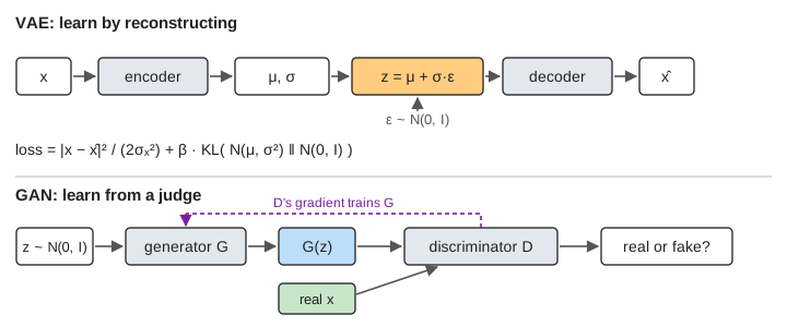
A generative model learns to make new data that looks like its training data. Both models on this page do it the same way at the end: draw a random latent z from the normal distribution N(0, I) and push it through a network. They differ in how that network is trained. A VAE (variational autoencoder) learns to compress each training point into a small Gaussian and decode it back. A GAN (generative adversarial network) never compresses anything: a generator and a discriminator play a game against each other.
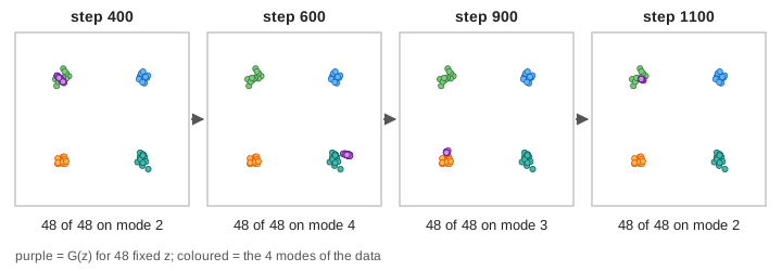
On the canvas the data is 48 points in 2D, 12 around each of 4 centres (±1.5, ±1.5): four modes, coloured 1 to 4. All four networks are tiny (2 inputs, 16 tanh units, a few outputs) and are trained for real in your browser with backpropagation and the Adam optimizer, from fixed random seeds, so every run gives the same numbers. The purple dots are always the same 48 latents z passed through the current decoder (VAE) or generator (GAN), so you see the models change, not the random draws. The bars under each plot count how many of those samples land on each mode, and how many land between modes.
The VAE: encoder, latent Gaussian, decoder
The encoder reads a point x and outputs two things per latent dimension: a mean μ and a log variance log σ². Together they describe a small Gaussian q(z | x) = N(μ, σ²): the region of latent codes that stand for x. The latent plot shows μ for every training point, in its mode's colour. A code z is drawn from that Gaussian, and the decoder turns it back into a point x̂, the reconstruction. (Demo 1: one training step of each, walked through.)
The reparameterization trick
Training needs the gradient of the loss with respect to μ and σ, but "draw z at random from N(μ, σ²)" has no gradient. The fix is to move the randomness out of the network:
ε ~ N(0, I)           // plain noise, an input like any other
z = μ + σ · ε         // differentiable in μ and σ
∂z/∂μ = 1,  ∂z/∂σ = ε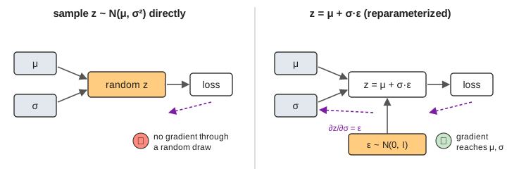
In the walk-through, the black cross in the latent plot is μ ± σ and the orange dot is the sampled z.
The loss: reconstruction + KL
For each point the VAE minimizes
loss = |x − x̂|² / (2σₓ²)  +  β · KL( N(μ, σ²) ‖ N(0, I) )
KL   = ½ Σ ( μ² + σ² − 1 − log σ² )                    // per latent dimension
The reconstruction term (σₓ² = 0.1 here) wants x̂ close to x. The KL divergence wants every q(z | x) close to the prior N(0, I): means near 0, spreads near 1. The two pull against each other. The KL term is what lets you generate: because the codes of all training points fill the prior, a random z from N(0, I) lands on some code and decodes to data. With β = 0 the encoder spreads the codes far out and shrinks σ; the reconstructions are better, but most random z fall in empty latent space and decode to points between or outside the modes. (Demo 4: VAE without the KL term.) The sum of the two terms is the negative ELBO, a lower bound on the log likelihood of the data.
With β = 1 the VAE covers all four modes but puts many samples between them: in a 2D latent space the codes of neighbouring modes touch, and the decoder blends them. On images this shows as the typical blur of VAE samples. (Demo 2: train both for 600 steps.)
The GAN game and alternating updates
The discriminator D(x) outputs the probability that x is real. The generator G(z) wants its fakes to be scored as real. Training alternates two steps:
- D step: on a batch of real points and a batch of fakes, minimize −log D(x) − log(1 − D(G(z))). The shading of the GAN plot is D(x): darker means "real".
- G step: with D frozen, minimize −log D(G(z)) (the non-saturating loss). The gradient flows back through D into G, so G moves its points uphill on D's shading.
G never sees a training point; all it knows about the data comes through D's gradient. At the ideal end of the game G matches the data, D can't tell them apart and outputs ½ everywhere: D loss 2·ln 2 ≈ 1.39 and G loss ln 2 ≈ 0.69. In practice the losses hover near those values and say little about sample quality, which is why the page counts samples per mode instead.
Mode collapse
Set G steps per D step to 5 and G gets five moves against a discriminator that stands still. The best answer to a fixed D is to put every sample at the one place D likes most, so G drops the other modes: mode collapse. D then learns that this mode is full of fakes and lowers its score there, and G runs to another mode. The samples stay sharp but cover one mode at a time and hop around. (Demo 3: mode collapse, 5 G steps per D step.)
Real fixes change the game rather than the step counts: minibatch discrimination (D sees whole batches, so it notices when all fakes look alike), unrolled GANs, Wasserstein GANs with a gradient penalty, and spectral normalization.
VAE vs GAN at a glance
| VAE | GAN | |
|---|---|---|
| networks | encoder + decoder | generator + discriminator |
| latent code for a real x | yes, N(μ, σ²) from the encoder | no encoder |
| loss | reconstruction + KL, one number to minimize | a two-player game, two losses |
| training | stable, the loss falls steadily | can oscillate, needs balancing |
| samples | cover every mode, but blurry / between modes | sharp, but may miss modes |
| typical failure | blur; with too much KL, ignoring z | mode collapse, unstable training |
Both ideas live on in today's models. Stable Diffusion uses a VAE to compress images into a small latent space and runs a diffusion model there; its decoder is often fine-tuned with a GAN-style discriminator loss to make it sharper. The networks themselves are ordinary neural networks trained with backpropagation.
What the page leaves out
Real VAEs and GANs work on images with convolutional networks, latent spaces of 100s of dimensions and minibatches drawn from millions of examples; here everything is 2D and full-batch. The page leaves out conditional models, β-VAE disentanglement, posterior collapse with strong decoders, VQ-VAE, Wasserstein and other GAN losses, progressive and StyleGAN architectures, and the evaluation metrics (FID, precision and recall of samples) that replace the simple "samples per mode" count used here.