Quantity Theory of Money Visualization

The idea: money that keeps moving

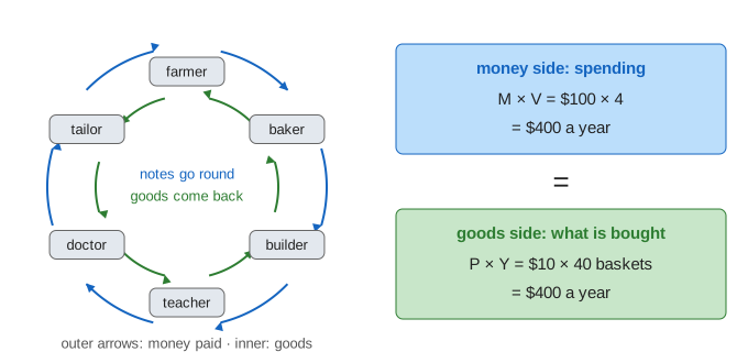
A dollar is not spent once. You pay the baker, the baker pays the farmer, the farmer pays the builder, and the same note has paid for three things. The money stock M is how many dollars exist. The velocity V is how many times, on average, each dollar is spent on goods and services in a year. So M × V is total nominal spending in the year.

Every purchase has a price and a quantity. Add up all of them and you get the price level P times real output Y, which is nominal GDP. Spending and what is bought are the same transactions counted from two sides, so

M \times V = P \times Y

This is the equation of exchange (Irving Fisher, 1911). The page starts with M = $100 in ten $10 notes, V = 4, so spending is $400. That buys Y = 40 baskets of goods at P = $10 a basket. (Demo 1: one year of MV = PY shows the notes going round four times.)

Banknotes worth M = $100 go round a ring of traders 4 times a year, so spending MV is $400. Goods come back the other way: 40 baskets at $10 each, so PY is $400. The two sides are equal. — Money goes one way, goods go the other: what is paid (M × V) always equals what is bought (P × Y).

From identity to theory

As written, MV = PY is always true: V is usually measured as nominal GDP divided by M. It becomes a theory (the quantity theory of money) when we add two claims about what moves on its own:

V is fairly stable: it depends on payment habits and technology (how often people are paid, cards, bank accounts), which change slowly.
Y is set by real things: workers, machines, technology. In the long run it grows at its own pace, called potential output Y*, whatever M does.

If V and Y do not respond to M, then more money can only mean higher prices. The page draws Y* as the row of baskets the economy can make, and the market-clearing price as P* = MV / Y*.

Inflation = money growth − output growth

Write the identity in growth rates: (1 + %ΔM)(1 + %ΔV) = (1 + %ΔP)(1 + %ΔY), or for small rates

%ΔM + %ΔV \approx %ΔP + %ΔY

With V steady, inflation ≈ money growth − output growth. The goods market panel shows each year's four growth rates, and the ledger keeps every year.

Demo	%ΔM	%ΔV	%ΔY	Result after 5 years
2: money +10%/yr, output flat	+10%	0	0	P $10 → $16.11, inflation 10.0% every year
3: money and output +4%/yr	+4%	0	+4%	P stays $10.00, Y 40 → 48.67
7: hyperinflation	+50% … +500%	4 → 12	−5%/yr	M ×216, P ×837

This is why central banks watch money and credit growth, and why "too much money chasing too few goods" is the classic description of inflation. Over long periods and across countries, high money growth and high inflation go together very closely.

Velocity is not constant

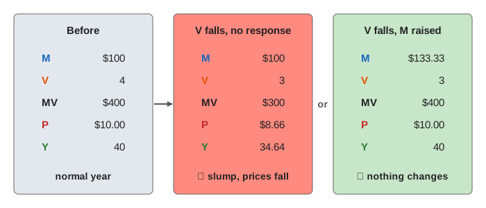
The weak point of the simple theory is V. When people are scared, they keep cash and bank deposits instead of spending them: money is hoarded, and V falls. In the page, notes that are hoarded move to the "idle money" box and skip the rounds of payments. With V = 3 a quarter of the money sits idle, so the same $100 only buys $300 of goods.

If prices are slow to fall, that lost spending means fewer baskets are sold: a slump (Demo 4: money hoarded: Y falls from 40 to 34.64 in the first year, P from $10 to $8.66, then prices keep falling slowly and output creeps back). A central bank can offset the fall in V by raising M: in Demo 5 M rises by a third to $133.33, MV stays at $400, and P and Y do not move at all.

That is roughly what happened in 2008 and in 2020. The Fed's balance sheet and, in 2020, the M2 money stock grew very fast, yet inflation stayed low at first, because the velocity of M2 fell sharply (it is published as M2V in FRED). Large money growth with low inflation is not a contradiction of MV = PY; it is a fall in V.

Before: M $100 times V 4 is $400, buying 40 baskets at $10. V falls to 3. Without the central bank: M $100 times 3 is $300, P $8.66, Y 34.64, a slump. With the central bank raising M to $133.33: $133.33 times 3 is $400, P $10, Y 40, nothing changes. — A fall in velocity cuts spending unless the central bank adds money to make up for it.

Short run and long run: sticky prices and neutrality

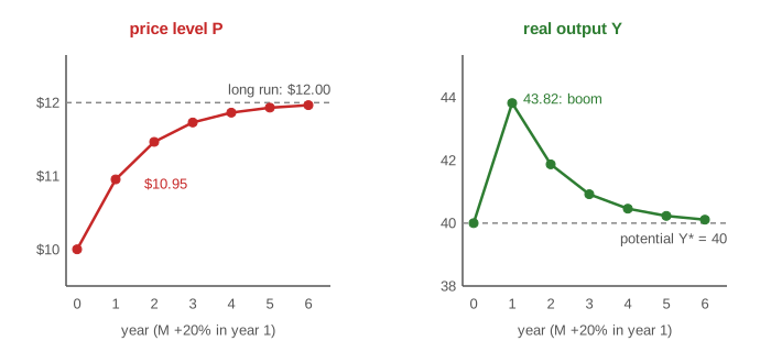
Prices do not all change at once. Menus, wages and contracts are reset only now and then. The page's sticky prices setting lets half of the firms reset to P* each year while the other half keep last year's price (plus the inflation they expect when the policy has not changed): P = √(P* × P_last × (1 + expected inflation)). Output is then whatever spending buys at that price: Y = MV / P.

In Demo 6: one-time +20% money, M goes from $100 to $120 and spending from $400 to $480. In year 1 prices rise only to $10.95, so $480 buys 43.82 baskets: a boom. Each year more firms catch up; by year 6 P is $11.97 and Y is back to 40.11. In the end money has raised prices by 20% and changed nothing real: money is neutral in the long run but not in the short run. With flexible prices (the "long run" setting) the same jump moves P straight to $12.00.

After M rises 20% in year 1, the price level climbs from $10 through $10.95, $11.47, $11.73 and $11.86 towards $12, while output jumps from 40 to 43.82 and falls back through 41.87 and 40.92 towards 40. — With sticky prices a money surprise first moves output, then prices catch up and output returns to potential.

Expectations matter here. A money growth rate that has been running unchanged is expected, so firms build it into their prices and it barely moves output; it is the surprise that causes the boom or the slump. That is why a steady +10% a year (sticky prices, any number of years) ends with 10% inflation and Y at potential, not with a permanent boom.

Hyperinflation

When a government pays its bills by printing money, M can grow 50%, 100% or 500% a year. People then try to get rid of money before it loses value: they spend wages the same day, buy goods to hold, or switch to foreign currency. V rises, and output usually falls as normal trade breaks down. Both push prices up even faster than money. In Demo 7, M grows 216-fold in five years, but because V rises from 4 to 12 and Y falls from 40 to 30.95, prices rise 837-fold, and inflation in the last year is 658%. The central bank also has to print bigger notes: the page's notes go from $10 to $20, $100, $500 and then $2k, as real hyperinflations moved to ever larger denominations (Germany 1923, Zimbabwe 2008).

A hyperinflation ends when money growth stops, usually with a new currency and a credible budget. Velocity then falls back, so in the first months the central bank can let M grow without restarting inflation.

See also the circular flow of money (who pays whom across households, firms and government), monetary policy transmission (how a rate change reaches spending), and liquidity preference (why people choose to hold money rather than bonds, which is what moves V).

What the page leaves out

The page has one kind of money and one good. Real economies have several measures of money (currency, M1, M2), most of it created by banks when they lend, not printed by the central bank, and the central bank mostly steers an interest rate rather than M directly. Velocity responds to interest rates and to financial innovation, not only to fear. Output growth and expectations are set by hand here; in reality they respond to policy, and price setting is far more varied than "half the firms reset each year".