The idea: slice the surface, take one slope
A function of two variables, z = f(x, y), is a surface. At a point P = (a, b) it has no single slope: walking east is not the same as walking north. So take one direction at a time. Freeze y = b. The vertical plane y = b cuts the surface in a curve, z = f(x, b), and that curve is an ordinary graph of one variable x. Its slope at x = a is the partial derivative
∂f/∂x (a, b) = limh→0 (f(a + h, b) − f(a, b)) / h
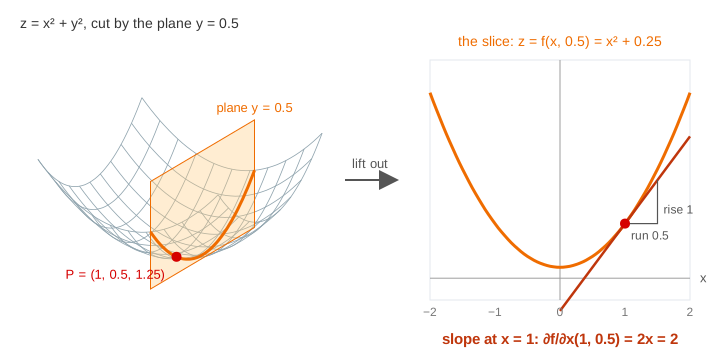
Freeze x = a instead and the slice z = f(a, y) gives the other partial derivative, ∂f/∂y. Other names: fx, fy, ∂z/∂x. On the canvas each slice takes four steps: the vertical plane appears, it cuts the surface, the cut is lifted out onto its own 2D graph, and the tangent line with its run and rise is drawn. (Demo 1: slice the bowl, take the x-slope)
Computing one: treat the other variable as a constant
Freezing y on the picture is the same as treating y as a number in the formula. Then the usual rules of one-variable calculus apply.
| f(x, y) | ∂f/∂x (y constant) | ∂f/∂y (x constant) |
|---|---|---|
| x2 + y2 | 2x | 2y |
| x2 − y2 | 2x | −2y |
| 3e−(x2 + y2)/2 | −x·f(x, y) | −y·f(x, y) |
| sin x · cos y | cos x · cos y | −sin x · sin y |
| x2y | 2xy | x2 |
For the bowl at P = (1, 0.5) the x-slice is z = x2 + 0.25: the 0.25 = y2 is just a constant that shifts the curve up, so its slope is 2x = 2. The page checks every slope against the difference quotient with h = 0.01: (f(1.01, 0.5) − f(1, 0.5)) / 0.01 = 2.01. The chain rule works the same way for the hill: d/dx of e−(x2 + y2)/2 is −x times itself. More on that rule: The Chain Rule.
Two slices, two slopes
The two slopes at one point are usually different, and can have opposite signs.
- Saddle z = x2 − y2 at (1, 1): the x-slice x2 − 1 climbs with slope 2, the y-slice 1 − y2 falls with slope −2. (Demo 3: saddle: one slope up, one down)
- Wave sin x · cos y at (1, 1): fx = cos 1 · cos 1 = 0.29 (gentle rise), fy = −sin 1 · sin 1 = −0.71 (steeper fall). (Demo 5: wave: two different slopes)
- Hill at (1, 0): the y-slice runs around the hill, across its side, so fy = 0 while fx = −1.82 points straight downhill.
Put together as a vector, (fx, fy) is the gradient ∇f. It points straight uphill, at right angles to the level curve through P (see Level Curves and Contour Maps), and Gradient Descent walks against it.
The tangent plane
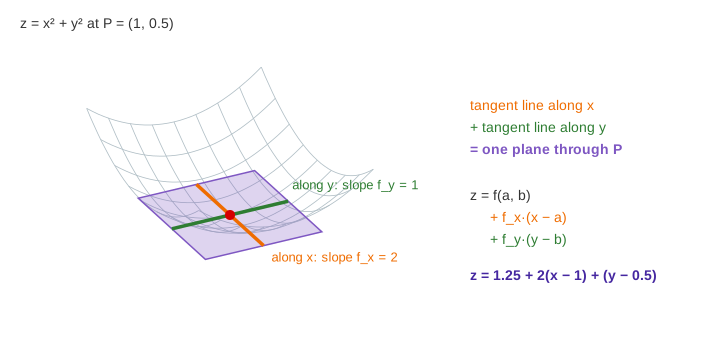
The two tangent lines both pass through P, so they lie in one plane. Moving Δx along x raises it by fxΔx, moving Δy along y raises it by fyΔy, so
z = f(a, b) + fx(a, b)·(x − a) + fy(a, b)·(y − b)
For the bowl at (1, 0.5): z = 1.25 + 2(x − 1) + (y − 0.5). Near P the plane hugs the surface: at (1.2, 0.6) the plane says 1.75 and f says 1.80. This is local linearity in two variables: zoom in on a smooth surface and it looks flat. (Demo 2: both slopes and the tangent plane) For a surface given as F(x, y, z) = 0 instead of a graph, the same plane comes from ∇F: Tangent Planes to Quadric Surfaces.
A flat tangent plane: top, bottom or saddle
When fx = fy = 0 both slices are flat at P and the tangent plane is horizontal. That happens at the top of the hill (z = 3), the bottom of the bowl and the middle of the saddle. The two first derivatives cannot tell these apart: the saddle's x-slice has a bottom at P while its y-slice has a top. The second-derivative test does that job, see Critical and Singular Points. (Demo 4: top of the hill: both slopes 0)
See also Level Curves and Contour Maps, The Derivative as a Limit, Lagrange Multipliers and Hyperbolic Paraboloid.
What the page leaves out
Directional derivatives in other directions, second and mixed partials fxx, fxy (and Clairaut's theorem fxy = fyx), functions of three or more variables, differentiability (a function can have both partial derivatives at a point and still no tangent plane), and hidden-line removal in the 3D view.