The idea: the average slope is reached somewhere
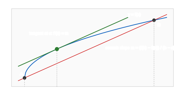
Join the two ends of a curve, A = (a, f(a)) and B = (b, f(b)), with a straight line, the secant. Its slope is the average rate of change m = (f(b) − f(a)) / (b − a). The Mean Value Theorem says that if f is continuous on [a, b] and differentiable on (a, b), then at some point c strictly between a and b the tangent has exactly that slope:
f′(c) = (f(b) − f(a)) / (b − a)
In pictures: somewhere the tangent is parallel to the secant.
Finding c: slide the secant
Copy the secant and slide the copy sideways without turning it. The last place it still touches the curve is a point where the curve does not cross it, so it is a tangent there, with slope m. That point is c. For √x on [0, 4], m = (2 − 0) / 4 = 1/2 and f′(x) = 1 / (2√x) = 1/2 at c = 1. (Demo: √x on [0, 4])
Why must this happen? Look at the gap g(x) = f(x) − (secant at x). It is 0 at a and at b. A continuous g on [a, b] has a highest and a lowest point, and if one of them is inside (a, b), the slope of g is 0 there, which means f′(c) = m. The sliding line is just the level of that highest or lowest point.
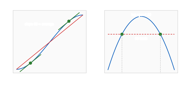
The theorem promises at least one c, not exactly one. x³ − 3x on [−2, 2] has m = 1 and two points with 3c² − 3 = 1, at c = ±2/√3 ≈ ±1.1547: slide up to one, down to the other. (Demo: x³ − 3x)
| f on [a, b] | m | c with f′(c) = m |
|---|---|---|
| √x on [0, 4] | 1/2 | 1 |
| x³ − 3x on [−2, 2] | 1 | −1.1547 and 1.1547 |
| sin x on [0, π] | 0 | π/2 |
| eˣ on [0, 1] | e − 1 ≈ 1.718 | ln(e − 1) ≈ 0.5413 |
Rolle's theorem: the flat case
When f(a) = f(b) the secant is horizontal, m = 0, and the theorem says there is a horizontal tangent somewhere in between: f′(c) = 0. This special case is Rolle's theorem, and the general theorem is proved from it by subtracting the secant (the gap g above has g(a) = g(b) = 0). For sin x on [0, π] the flat tangent is at the top, c = π/2. (Demo: Rolle)
The speed story
A car drives 120 km in 2 hours. Its average speed is 60 km/h, the slope of the secant on the position graph. The car's speed at each moment is the slope of the tangent, the number on the speedometer. The theorem says: at some instant the speedometer reads exactly 60. In the demo the car starts and ends at rest and peaks at 90 km/h, so it passes 60 twice, at t ≈ 0.42 h speeding up and t ≈ 1.58 h slowing down. (Demo: car trip)
This is how average-speed cameras work: if your time between two cameras gives an average above the limit, then at some moment you were going above it.
When the hypotheses fail
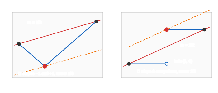
Both conditions matter. If f has a corner (not differentiable) or a jump (not continuous), the sliding line can last touch at that bad point, where there is no tangent at all.
- |x| on [−1, 2]: m = (2 − 1) / 3 = 1/3, but the slope of |x| is −1 or +1 everywhere, never 1/3. The line last touches at the corner (0, 0). (Demo: fails for |x|)
- A step, 0 for x < 1 and 1 for x ≥ 1, on [0, 2]: m = 1/2, but the slope is 0 wherever it exists. The line touches only the top of the jump, and slides through the hole at (1, 0). (Demo: fails for a jump)
Why it matters
- If f′(x) = 0 everywhere on an interval, f is constant: any two points have m = f′(c) = 0. So two antiderivatives differ by a constant, which the Fundamental Theorem of Calculus relies on.
- If f′ > 0 on an interval, f is increasing; this is the reason the sign of f′ tells where a graph rises (Derivative Graphs).
- Error bounds: |f(b) − f(a)| ≤ (max |f′|) · |b − a|. It bounds the error of Riemann sums, Euler's method and the remainder of Taylor series.
- Local linearity says f(x + h) ≈ f(x) + f′(x)·h; the theorem makes it exact: f(x + h) = f(x) + f′(c)·h for some c between x and x + h.
See also the derivative as a limit (where the tangent slope comes from) and Limits (continuity).
What the page leaves out
The c values come from solving f′(c) = m by hand, not from a numeric search. The page does not prove that a continuous function on [a, b] has a maximum (the extreme value theorem), and it does not cover Cauchy's mean value theorem (used for L'Hôpital's rule), the mean value theorem for integrals, or functions of several variables.