The idea: the best point is where a level curve just touches
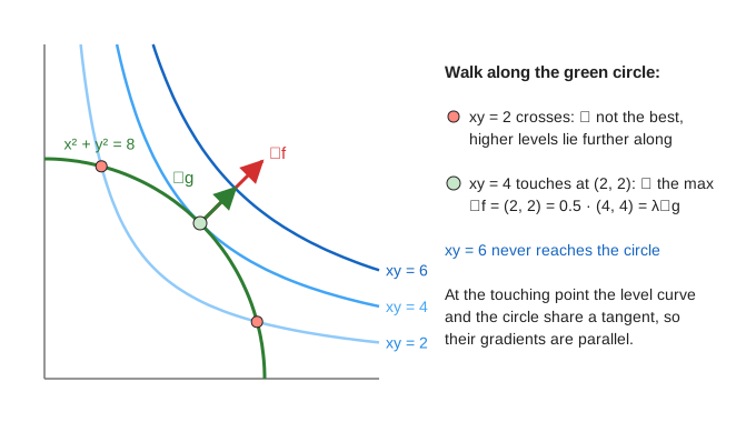
You want the largest value of f(x, y), but you may only stand on a curve g(x, y) = c: a budget, a fence, a fixed amount of material. Draw the level curves of f and walk along the constraint. While the level curve through you crosses the constraint, higher levels lie ahead, so you can still do better. You stop where a level curve only touches the constraint. There the two curves have the same tangent, so their gradients are parallel: ∇f = λ∇g. The page uses one function throughout, f(x, y) = xy.
The gradient
The gradient collects the two partial derivatives: ∇f = (∂f/∂x, ∂f/∂y). For f = xy that is (y, x), so at P = (1, 2) it is (2, 1). Three facts make it useful:
- it points in the direction in which f grows fastest;
- its length |∇f| is that fastest slope: √(2² + 1²) ≈ 2.24 at (1, 2);
- it is perpendicular to the level curve through the point.
The last one is easy to see: along the level curve f does not change, so all of the change is across it (Demo: gradient ⟂ level curves). Where ∇f = (0, 0) the point is critical: for xy that is only (0, 0), a saddle, where the level f = 0 is the two axes crossing (Demo: saddle point).
The directional derivative ∇f · u
Pick a unit direction u = (cos θ, sin θ). The slope of f in that direction is the directional derivative
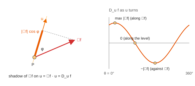
Duf = ∇f · u = |∇f| cos φ,
where φ is the angle between ∇f and u. It is the length of ∇f's shadow on u. At (1, 2) with θ = 30°: 2 · 0.87 + 1 · 0.5 = 2.23. As u turns, cos φ makes Duf a cosine of height |∇f| (Demo: directional derivative):
| direction u | φ | Duf |
|---|---|---|
| along ∇f | 0° | |∇f| (steepest ascent) |
| along the level curve | 90° | 0 |
| against ∇f | 180° | −|∇f| (steepest descent, what gradient descent follows) |
Walking the constraint
On the constraint, P can only move along the curve, in the direction of its unit tangent T. The slope of f along the walk is ∇f · T. If it is positive, walk on; if negative, walk back. At a maximum or minimum it must be 0, so ∇f is at right angles to the constraint. But ∇g is at right angles to the constraint too (the constraint is a level curve of g). Two vectors at right angles to the same line are parallel:
∇f = λ∇g, g(x, y) = c.
The number λ is the Lagrange multiplier. These are three equations for x, y and λ.
Solving: xy on the circle x² + y² = 8
∇f = (y, x) and ∇g = (2x, 2y), so y = 2λx and x = 2λy. Multiply them: xy = 4λ²xy, so λ = ±½ (or xy = 0, which forces x = y = 0, off the circle). λ = ½ gives y = x, and x² + y² = 8 gives (2, 2) and (−2, −2) with f = 4: the maxima. λ = −½ gives y = −x: (2, −2) and (−2, 2) with f = −4, the minima. On the circle f = 8 cos θ sin θ = 4 sin 2θ, which the chart draws as P walks (Demo: Lagrange on the circle).
On the line x + y = 4, ∇g = (1, 1), so y = λ and x = λ: x = y = 2, λ = 2, f = 4. That is the only tangency and it is a maximum; there is no minimum, because f = x(4 − x) falls without end (Demo: Lagrange on the line). Lagrange's equations find candidates; you still compare them, and check that a best point exists at all.
What λ means
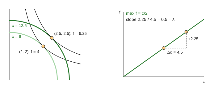
λ is the rate at which the best value changes when the constraint is loosened: d(max f)/dc = λ. On x² + y² = c the best point is x = y = √(c/2), so max f = c/2 and the slope is ½ = λ. Going from c = 8 to c = 12.5 raises the max from 4 to 6.25: 2.25 / 4.5 = 0.5 (Demo: λ = how fast the max grows). Economists call λ a shadow price: what one more unit of budget is worth.
Where it is used
- Economics: maximize utility on a budget line; λ is the marginal utility of money.
- Physics: constrained motion (a bead on a wire); λ is the force of the constraint.
- Machine learning: the support vector machine is solved through its Lagrange dual, and the support vectors are the points with λ > 0.
- Statistics: the largest variance direction of PCA is ∇(uᵀAu) = λ∇(uᵀu), the eigenvector equation Au = λu.
See also Level Curves and Contour Maps for how the contour map is made, Vectors and the Dot Product for the projection behind ∇f · u, and Gradient Descent, which follows −∇f without a constraint.
What the page leaves out
More variables and several constraints (∇f = λ₁∇g₁ + λ₂∇g₂), inequality constraints and the Karush–Kuhn–Tucker conditions, the second-order test with the bordered Hessian that tells a max from a min without comparing values, points where ∇g = 0 (the method needs ∇g ≠ 0), and numerical methods such as penalty and augmented Lagrangian methods. The page also checks only 15° stops on the circle; the exact answer comes from the equations.