The idea: one price level, one output, two curves
A whole economy can be squeezed into two numbers: the price level P (an index of what things cost, 100 at the start) and real output Y (how much is produced). The AD–AS model finds them where two curves cross. Aggregate demand (AD) says how much people, firms, the government and foreigners want to buy at each price level. Short-run aggregate supply (SRAS) says how much firms produce at each price level this year. A third line, long-run aggregate supply (LRAS), stands straight up at potential output Y*: what the economy makes with normal employment.
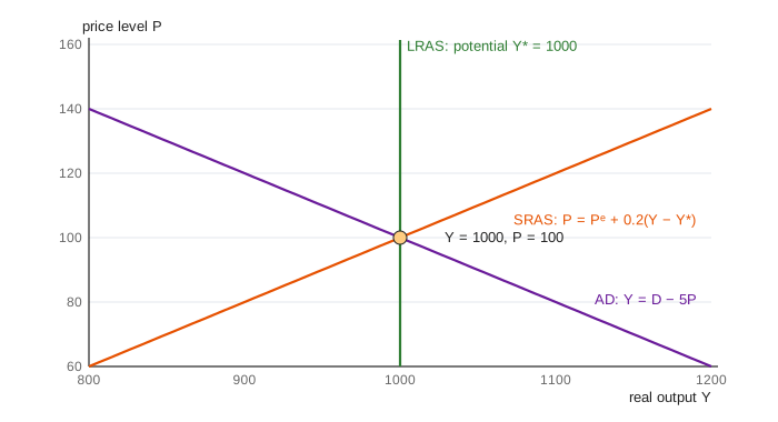
The page uses small numbers you can check by hand. AD is Y = D − 5·P with a spending shifter D = 1500. SRAS is P = Pᵉ + 0.2·(Y − Y*) + z. Potential output is Y* = 1000. Year 1 starts at Y = 1000, P = 100.
Why AD slopes down
With the same money spending, a higher price level buys fewer real goods. It also raises interest rates: people need more money for their purchases, so they sell bonds and the rate goes up (see Liquidity Preference). And it makes exports dearer. All three cut real purchases, so AD slopes down.
Anything that changes spending at a given price level shifts the whole curve: government purchases, taxes, the money supply and interest rates, confidence, or foreign demand. On the page all of this is the shifter D. Raise Demand adds 100 to D, and the curve moves 100 to the right.
Why SRAS slopes up: wage contracts
Wages are set in advance, for about a year, based on the price level people expect, Pᵉ. If prices turn out higher than expected, the real wage W/P falls. Labour is cheap for firms, so they hire more and produce more. If prices turn out lower, the real wage is high and firms cut back. That is why, within a year, higher prices go with more output. The "Wage contracts" panel shows W = Pᵉ next to the actual P.
Two things move SRAS. New contracts move it up or down: next year's Pᵉ is this year's P. Cost shocks move it too: an oil price jump adds z = +20 to the prices firms need at every output level.
Potential output, the output gap and Okun's law
The output gap is (Y − Y*) / Y*. When output is above potential, more people are working than normal, and unemployment falls below its natural rate. Okun's law puts a number on it. The page uses u = 5% − 0.5 × gap%, so a 5% boom gives 2.5% unemployment and a 5% slump gives 7.5%. Inflation is the yearly change in P.
Demand shocks: short run vs long run
Say D rises by 100. At the old price level of 100, people want to buy 1100 but firms make 1000. Prices rise until the two meet, at P = 110 and Y = 1050: a boom with unemployment at 2.5% (Demo: demand boom). Output and prices moved the same way.
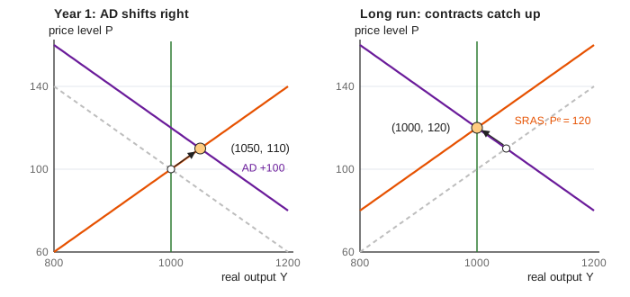
Next year, workers who saw prices of 110 sign contracts at W = 110. SRAS shifts up, output slips to 1025 and prices rise to 115. Each year the gap halves, and the economy ends at Y = 1000 with P = 120. In the long run, demand changes only the price level. A slump runs the same way in reverse: Y = 950 and P = 90 in year 1, then wages and prices fall slowly back toward Y* (Demo: demand slump).
Supply shocks and stagflation
An oil shock shifts SRAS up by 20 for one year. Prices rise to 110 while output falls to 950 (Demo: oil shock). Prices and output now move opposite ways: inflation and unemployment rise together. This is stagflation, as in 1974 and 1979.
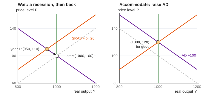
Policy has no good option. If it waits, the shock fades and wages adjust, but slowly: output is back near 998 only after five years. If it accommodates by raising demand by 100 in the same year, output stays at 1000 but prices jump to 120. Next year's contracts lock that level in (Demo: oil shock accommodated). The Phillips curve page shows the same choice as inflation against unemployment.
A lasting rise in productivity is the friendly supply shock. Potential output moves to 1100 and, over time, prices fall to 80. In year 1 output only gets to 1050, though. Prices fell below what the contracts expected, so the real wage is high (Demo: productivity boom).
Self-correction is slow: the case for stimulus
Left alone, the economy returns to potential: wage contracts adjust and SRAS shifts. Here half of the gap closes each year, so a slump of 5% of output takes about five years to close. In real economies wages fall even more slowly than they rise. Keynes's answer was to shift AD back instead. Demo: slump met by stimulus offsets the fall in demand within the same year, and output never leaves 1000. The Monetary Transmission page shows how a central bank moves demand. Fiscal policy moves it directly.
What the page leaves out
Real AD and SRAS are not straight lines, and nothing here grows over time. Expectations are purely backward-looking (last year's price), and all wages are reset together once a year. In reality contracts overlap, and some prices are sticky for other reasons. Potential output has no investment or capital stock behind it, money and interest rates sit inside the single shifter D, and there are no imports, exchange rates or debt. Modern models (New Keynesian DSGE) add forward-looking expectations and an explicit central bank rule.