The idea: merge the closest pair, again and again
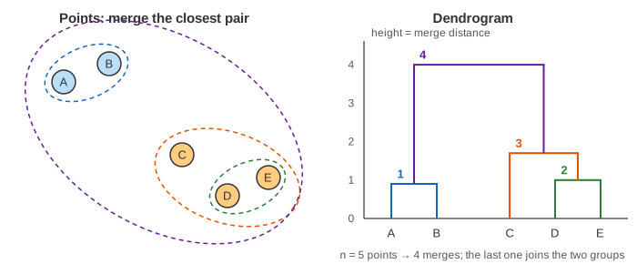
Agglomerative hierarchical clustering starts with every point as a cluster of its own. Then it repeats one move: find the two clusters that are closest together and merge them. With n points that takes n − 1 merges, and at the end everything is one cluster. You do not choose the number of clusters up front. The result is a whole family of clusterings, one for every number from n down to 1, drawn as a tree called the dendrogram.
The algorithm
- Make one cluster per point.
- Compute the distance between every pair of clusters.
- Merge the pair with the smallest distance. Record the merge and its distance.
- Repeat from step 2 until one cluster is left.
On the canvas each merge takes three Steps: the closest pair is ringed and joined by an orange line,
a box with its distance d appears; the box flies to the dendrogram; then the ∩ is drawn and the two
clusters take one colour. The narration also names the runner-up pair, so you can see how close the race was.
(Demo 1: build the dendrogram: 11 merges for 12 points, the first ones inside the blobs at heights
1.03 to 1.85, the last two between blobs at 5.64 and 5.96.)
Linkage: what "closest" means for two clusters
The distance between two points is clear. Between two groups of points there is a choice, called the linkage:
| Linkage | Distance between clusters A and B | Effect |
|---|---|---|
| single | the closest pair: min d(a, b) | follows chains; can glue groups through a thin line of points |
| complete | the farthest pair: max d(a, b) | compact, similar-diameter clusters; sensitive to outliers |
| average (UPGMA) | the mean of all |A|·|B| point distances | between single and complete |
| Ward | the increase in within-cluster sum of squares; scipy draws it as √(2·|A|·|B| / (|A|+|B|)) · ‖cA − cB‖ | round clusters of similar size, like K-Means; the default in scikit-learn |
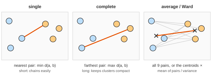
The page joins the pair that defines the distance with an orange line: the two nearest points for single linkage, the two farthest for complete, and the two centroids (orange squares) for average and Ward, where the distance is a mean or a variance and no single pair defines it. With all four linkages the merge heights never go down from one merge to the next, so the dendrogram has no crossings. (Centroid and median linkage can produce such inversions; the page leaves them out.)
Reading and cutting the dendrogram
The height of a ∩ is the distance at which its two branches were joined. To get k clusters, draw a horizontal line that crosses exactly k vertical branches: everything hanging below one crossing is one cluster. A long vertical stretch with no merges means the groups below it are well separated, so the biggest gap between two consecutive merge heights is a natural place to cut.
- Demo 2: cut at the biggest gap: average linkage on the three blobs. The heights jump from 1.85 to 5.64, so the cut at 3.74 gives 3 clusters {A,B,C,D} {E,F,G,H} {I,J,K,L}.
- Demo 6: cut lower: at 1.64 the same tree gives 5 clusters; the blobs E–H and I–L each fall apart in two.
- Demo 5: Ward linkage: the same 3 clusters, but the top merges are at 11.14 and 12.01: Ward's heights are on a different scale, so compare the shape of the tree, not the numbers, across linkages.
Single linkage and chaining
Single linkage only needs one close pair to merge two clusters. On the second data set two groups are joined by a line of points about 1 apart, and that is enough: every merge happens between 0.82 and 1.36, the dendrogram has no gap, and cutting it into 2 clusters splits off just {A,B} from the other 12 points (Demo 3). This is chaining. Complete linkage on the same data needs every pair within the distance, so the long chain cannot merge cheaply: the top merge is at 8.02 after a jump from 4.36, and the cut gives the left group with half the bridge, {A,…,H}, and the right group {I,…,N} (Demo 4).
Single linkage is the same as building a minimum spanning tree with Kruskal's algorithm: sort the point pairs by distance and join with a union-find structure; each MST edge is one merge, and its length is the merge height. Cutting the dendrogram into k clusters = deleting the k − 1 longest MST edges.
Cost and how it compares
The page's naive version recomputes all pair distances after every merge: O(n³) time. Real libraries keep an n × n distance matrix and update only the new cluster's row with the Lance–Williams formula, which gives O(n²) memory and O(n²) to O(n² log n) time (SLINK for single linkage, nearest-neighbour chains for the others). Either way the n² matrix limits it to tens of thousands of points.
| Hierarchical | K-Means | DBSCAN | |
|---|---|---|---|
| number of clusters | chosen after, by the cut | K chosen before | follows from eps, minPts |
| result | a whole tree of nested clusterings | one partition | one partition + noise |
| shapes | depends on the linkage | round blobs | any shape |
| cost | O(n²) memory | O(n·K) per iteration | about O(n log n) with an index |
| deterministic | yes (ties aside) | depends on the start | yes, except some border points |
Like any distance-based method (see k-nearest neighbours), features on different scales should be standardized first, or the largest one decides every merge.
What the page leaves out
The data is 2-D with at most 14 points and Euclidean distance; other metrics (Manhattan, cosine, correlation for gene expression) plug into the same loop. The page does not show the distance matrix, the Lance–Williams update, centroid or median linkage and their inversions, divisive (top-down) clustering, connectivity constraints, or measures for picking the cut such as the cophenetic correlation or the silhouette score. Ties are broken by cluster order; with real data ties are rare but can change the tree.