k-means vs GMM Visualization | Hard vs Soft Clustering

The idea: two ways to split points into groups

Both methods on this page look for K = 3 groups in the same 60 points, and both start from the same three points. k-means keeps one centre per group and gives every point to its nearest centre, all or nothing. A Gaussian mixture model (GMM) says the data came from 3 bell-shaped normal distributions, each with its own centre, its own shape and its own size, and asks for every point how likely each of them is to have produced it. It is fitted with the EM (expectation–maximisation) algorithm.

Left: k-means, a point between two centroids goes 100 percent to the nearer one, with a straight border halfway between them. Right: a Gaussian mixture, the same point gets responsibilities 0.7 for the blue Gaussian and 0.3 for the red one, and the two Gaussians are drawn as ellipses of different shape. — k-means gives a point to one cluster; a Gaussian mixture gives it a share of every cluster.

The left panel is k-means, the right panel the GMM, on the same points. The background shading shows which cluster would win a new point at that spot. Pick a data set with data, then press One iteration to see one step of both, or Run to convergence.

Hard vs soft assignment

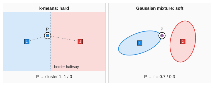
k-means makes a hard assignment: point P belongs 100% to cluster 1 and 0% to the others, even when it sits almost exactly between two centres. The GMM makes a soft assignment: the responsibility of Gaussian k for point x is

r_{k} = \frac{π_{k} N (x | μ_{k}, Σ_{k})}{\sum_{j} π_{j} N (x | μ_{j}, Σ_{j})}

The three responsibilities of a point add up to 1. On the canvas a point's colour is the mix of the three cluster colours in those proportions, so a purple point is half blue, half red. The stats line point P gives the numbers for the ringed point (Demo 1: one iteration, walked through).

The two steps, side by side

Both algorithms repeat the same two steps until nothing changes.

step	k-means	Gaussian mixture (EM)
assign / E-step	each point to its nearest centroid	responsibilities r for every point and Gaussian
update / M-step	centroid = mean of its points	mean μ = r-weighted mean; covariance Σ = r-weighted spread; weight π = (sum of r) / N
score that improves	inertia (SSE) Σ ‖x − μ‖², goes down	log-likelihood Σ log Σ_k π_k N(x \| μ_k, Σ_k), goes up
stops when	no point changes cluster	log-likelihood gains less than 0.001 per point
shape of a cluster	none stored (drawn: one circle for all)	an ellipse per cluster, from Σ

Each step can only improve its score, so both always stop, but at a local optimum that depends on where they started. That is why the page starts both from the same three points, one in each group. The covariance gets a small 0.01 added to its diagonal (reg_covar) so it never collapses onto a single point.

k-means is a special case

Take a GMM where every Gaussian has the same round covariance σ²I and the same weight 1/K. Then the responsibilities only depend on the distance to each mean. Now let σ shrink towards 0: the nearest mean takes a responsibility of 1 and all others 0, and the M-step becomes a plain mean. That is k-means. So k-means quietly assumes that every cluster is round and the same size. The circles on the left panel show that assumption: radius 2σ with σ² = SSE / (2N), the same for all three.

Where k-means fails

The border between two k-means clusters is the straight line halfway between their centroids. That is the right border only when the two groups are round and equally spread.

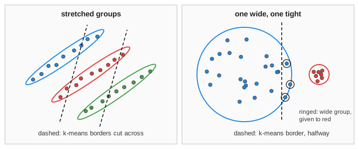
Two cases. Left: three long thin parallel groups; the k-means borders cut across them, the GMM ellipses lie along them. Right: a wide group next to a tight one; the k-means border halfway between the centres cuts off three edge points of the wide group, while a big and a small ellipse fit the two groups. — Straight halfway borders cut stretched groups and give a wide group's edge to its tight neighbour; fitted ellipses follow the data.

Stretched groups (Demo 3): three long thin groups side by side. k-means' lowest-SSE answer cuts across them and agrees with the true groups on only 37 of 60 points. The GMM stretches each Σ into a long ellipse and gets all 60.
Different sizes (Demo 4): a wide group of 36 next to two tight groups of 12. The halfway border gives the wide group's outer points to the tight ones (54 / 60). The GMM learns a wide Σ and a bigger weight π for the wide group (59 / 60).

On round groups of the same size (Demo 2) both agree on all 60 points: there the assumption is true and k-means is the cheaper choice. For groups that are not blobs at all (moons, rings), neither works; see DBSCAN.

Overlap and uncertainty

When two groups overlap (Demo 5), no method can be sure about the points in the middle. Both get about the same number right. The difference is what they say about it: k-means still puts every point 100% in one cluster, while the GMM gives 15 points less than 0.9 for any cluster. Those mixed-colour points are the ones a later step should treat with care, and the soft shading on the right shows the uncertain zone.

Choosing between them

	k-means	Gaussian mixture
output	one label per point	a probability per point and cluster
cluster shape	round, all the same size	any ellipse, any size and weight
cost per iteration	N·K distances	N·K densities plus K covariance fits
iterations here	usually a few	usually more (slow final gains)
risks	wrong shape assumption, bad start	bad start, a Gaussian collapsing on few points

In practice a GMM is often started from a k-means result, and both are run from several starts, keeping the best score (n_init). To learn the basic k-means loop step by step, and how its start and K matter, see K-Means Clustering.

What the page leaves out

K is fixed at 3; real use picks it with the elbow method, BIC or AIC. The start points are fixed, one per group, where libraries use k-means++ and several restarts. The GMM always uses full covariances; libraries also offer diagonal, spherical and tied ones. Real data has more than two dimensions, where the covariance has many more numbers to fit and EM needs more data and more regularisation.