The idea: a point gets the class of its neighbors
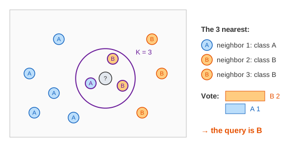
K-nearest neighbors (KNN) classifies a new point, the query, by looking at the K training points closest to it and taking a majority vote of their classes. There is no training step: the model is the stored training set. All the work happens when a query arrives.
The four steps
- Distances. Compute the distance from the query q to every one of the n training points.
- Sort them by distance (or keep only the K smallest).
- Take the K nearest. On the canvas a ball around q grows until it holds K points.
- Vote. The class with the most votes among those K is the answer.
The page has 14 training points in two classes. The table on the right lists every point's distance, then sorts it; the coloured rows at the top are the voters.
Choosing K
| K | what happens |
|---|---|
| 1 | the single nearest point decides alone; one mislabelled or unusual point flips every query near it |
| small, odd (3, 5, 7) | local, but a few noisy points are outvoted |
| even | with two classes the vote can tie, so a tie rule is needed |
| close to n | almost the whole training set votes, so every query gets the overall majority class |
Point #8 is a class B point sitting inside the A cluster. A query at (3.3, 2.6) is nearest to it, so K = 1 says B. With K = 5 four A points join and the answer becomes A, 4–1. (Demo: K = 1 vs K = 5)
At (7.5, 7), inside the B cluster, K = 3 says B 3–0. With K = 13 almost every point votes; there are only 6 B points, so A wins 7–6 even though the query is surrounded by B. Any K of 13 or more gives A everywhere. (Demo: K too large) In practice K is chosen by cross-validation: try several values and keep the one with the lowest error on held-out data.
Ties
At (4.9, 6.5) with K = 4 the vote is A 2, B 2. Something must break it. This page gives the win to the class of the
nearest neighbor (#14, class A). Other common rules: lower K by one, weight votes by 1/distance, or pick at random.
scikit-learn's KNeighborsClassifier returns the first class in label order. With two classes an odd K never ties;
K = 5 here gives A 3–2. (Demo: a tie vote) Points at exactly the same distance are another kind of tie;
here the lower point number comes first.
Distance metrics
| metric | formula (two features) | points at distance r from q |
|---|---|---|
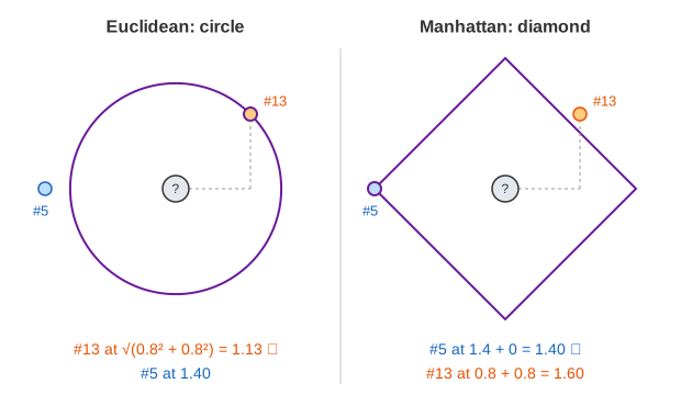
| Euclidean (L2) | √(Δx1² + Δx2²) | a circle |
| Manhattan (L1) | |Δx1| + |Δx2| | a diamond |
The shape of "near" changes which point is nearest. Point #13 is diagonally away from q = (6.7, 3.7), by (0.8, 0.8); point #5 is straight to the left, by 1.4. Euclidean: #13 at √(0.8² + 0.8²) = 1.13 is nearer, so K = 1 says B. Manhattan: #13 is at 0.8 + 0.8 = 1.60 and #5 at 1.40, so K = 1 says A. (Demo: Euclidean vs Manhattan)
Feature scaling
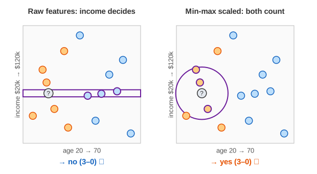
Distance adds up differences across features, so a feature measured in big numbers dominates. In the age & income data, age runs from 20 to 70 and income from $20,000 to $120,000. A $1,000 income difference counts as much as 1,000 years of age. The raw distance is really just the income difference: the query (age 28, $61,000) gets three neighbors with incomes near $61,000 who are all 48 or older and all said no.
Min-max scaling maps each feature to 0..1: x' = (x − min) / (max − min), with min and max taken from the training set. After scaling, one unit of age range and one unit of income range count the same, the ball becomes a circle on the plot again, and the three nearest are young buyers: yes, 3–0. (Demo: unscaled vs scaled features) Standardization ((x − mean) / standard deviation) is the other common choice. Either way the query must be scaled with the training set's numbers.
Cost and the curse of dimensionality
Training is free, but each query costs O(n·d) for n points with d features: every distance is computed. For large n, k-d trees and ball trees skip far regions, and approximate nearest neighbor indexes (HNSW, IVF) trade a little accuracy for a lot of speed — the same search that powers vector databases in retrieval-augmented generation. With many features every point ends up roughly equally far from every other, the curse of dimensionality, so KNN works best with few, meaningful, scaled features.
Variants
- Weighted KNN: each neighbor's vote counts 1/distance, so closer points matter more and ties are rare.
- KNN regression: predict the average of the K neighbors' values instead of a vote.
See also K-Means Clustering, which also uses distances to points but learns cluster centers without labels, and Decision Trees, another classifier that splits on one feature at a time and so does not need scaling.
Euclidean distance √(Δx² + Δy²) comes straight from the Pythagorean theorem.
Neighbourhoods within a radius are also the basis of DBSCAN density clustering.
Finding the K nearest among millions of points is done with approximate indexes such as HNSW.
To find the nearest neighbours without measuring every point, see KD-tree vs R-tree, which skip whole regions of the map.
See also Supervised vs Unsupervised vs Reinforcement Learning, where a labelled classifier, k-means and a reward learner train on the same points.
See also Support Vector Machine, which keeps only the few points on the edge of its margin instead of all training points.
What the page leaves out
Only two features and two classes, so the plot can show everything. No cross-validation, no weighted votes, no k-d tree or approximate search, no standardization (only min-max scaling), and no other metrics such as cosine or Minkowski with p ≠ 1, 2.