The idea: two ways to flatten points
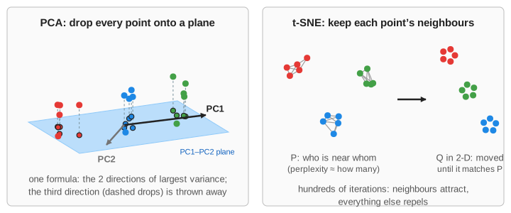
Data often has many numbers per item: pixels, word counts, gene levels. To look at it, you flatten it to 2-D. PCA (principal component analysis) does it with a linear projection: it picks the two directions in which the points spread the most and keeps only those coordinates. t-SNE (t-distributed stochastic neighbour embedding) does it by optimisation: it places points in 2-D at random, then moves them until each point's neighbours in 2-D are the same as its neighbours in the original space. The page runs both on the same 3-D points, one step each at a time, and scores the results.
PCA: keep the directions of largest variance
- Centre: subtract the mean from every point.
- Covariance: form the 3×3 matrix C = Σ x xᵀ / (N − 1).
- Eigenvectors of C are the principal components PC1, PC2, PC3, and each eigenvalue is the variance along it. The page shows each one's share: "PC1 57%, PC2 40%, PC3 3% (dropped)".
- Project: the new coordinates are x·PC1 and x·PC2.
That is a rotation followed by dropping an axis, so lengths along the kept plane are kept exactly. It has one answer, needs no settings, and also works on new points: project them the same way. See SVD and PCA in 2D for the covariance matrix and the principal axes step by step.
t-SNE: neighbours as probabilities
- P, in the original space. For each point i, a Gaussian over its distances to the others gives the probability p(j|i) that i "picks" j as a neighbour. Its width σᵢ is tuned per point by a binary search so that the perplexity of the row (e to the power of its entropy, roughly "how many neighbours") equals the setting. A point in a dense area gets a small σ, a point in a sparse area a large one. P is then made symmetric.
- Q, in 2-D. The same idea with a Student-t curve, q ∝ 1 / (1 + d²). Its heavy tail lets far-apart groups sit far apart without much cost.
- Move. Gradient descent on the mismatch KL(P‖Q): neighbours that are too far attract, points that are too close repel. The page runs 500 iterations, 50 per step, with the usual tricks: early exaggeration (P ×4 for the first 100 iterations, so groups form fast) and momentum.
The result depends on the random start, takes N² work per iteration (real tools use Barnes-Hut approximations), and has no formula for a new point. (Demo: another random start.)
When PCA puts groups on top of each other
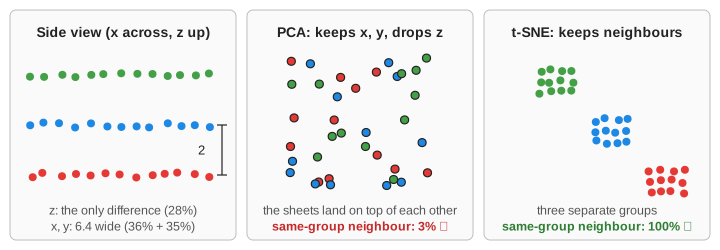
PCA keeps the directions with the most variance, not the ones that separate groups. In Demo: stacked sheets, three flat sheets are 6.4 wide in x and y and 2 apart in z. The widest directions are x and y, so PCA drops z, the only direction in which the sheets differ. They land on top of each other: only 3% of points have a nearest neighbour of their own colour. t-SNE only asks who is next to whom, and in 3-D almost all of a point's neighbours are on its own sheet, so it keeps them apart (100%).
The classic example is the Swiss roll, a sheet rolled up like a cake: PCA flattens the layers onto each other, t-SNE keeps neighbours along the sheet. It needs many more points than this page draws.
What t-SNE distances do not mean
t-SNE only matches neighbourhoods, and the heavy-tailed Q spreads everything else out. So in a t-SNE plot:
- Gaps between groups are not distances. In Demo: near and far groups, C is 5.9× farther from A than B is. PCA shows about the same (6.1×); t-SNE shows 2.6×.
- Group sizes are not spreads. C is 3.2× as spread out as A, yet in t-SNE it comes out about the same size (0.9×): each point's σ adapts to its local density.
- Small perplexity invents structure. With perplexity 2 each point listens to about 2 neighbours, and three real groups break into 16 small clumps (Demo: perplexity 2). Typical values are 5 to 50, and below the number of points in a group.
The scoreboard
| Row | What it measures | Who usually wins |
|---|---|---|
| neighbours kept | Of each point's 5 nearest neighbours in 3-D, how many are still among its 5 nearest in 2-D | t-SNE (it optimises exactly this) |
| nearest neighbour in the same group | Share of points whose nearest 2-D neighbour has their colour: are the groups kept apart? | t-SNE when groups differ in a small direction; a tie when they are far apart |
| distance correlation r | Pearson r between all 3-D distances and all 2-D distances: is the global shape kept? | PCA |
When to pick which
| PCA | t-SNE | |
|---|---|---|
| What it keeps | Global shape: directions, distances, variance | Local neighbourhoods |
| Speed | One eigenproblem; fine for millions of points | Hundreds of iterations, N² (or N log N with Barnes-Hut) |
| Same answer every run | Yes | No: depends on the random start |
| New points | Project them with the same PCs | Run it again |
| Settings | None (only how many components) | Perplexity, learning rate, iterations |
| Use it for | Compressing features, removing noise, a first look, a step before other models (and before t-SNE: reduce to ~50 PCs first) | Pictures of clusters in high-dimensional data: images, cells, word vectors |
Groups that a t-SNE picture shows are worth checking with a clustering method on the original data, such as K-Means or DBSCAN.
Common mistakes
- Reading cluster distances or sizes off a t-SNE plot. Neither is kept (Demo: near and far groups).
- Trusting one run or one perplexity. Try a few; real structure stays, accidents move.
- Thinking PCA failed because the picture looks mixed. PCA answers "where is the variance?". If the groups differ along a small direction, a mixed picture is the correct answer to that question.
- Forgetting to scale features before PCA. A feature measured in larger units gets more variance and takes over PC1.
What the page leaves out
The input is 3-D so you can see it; real data has tens to thousands of dimensions, where PCA is usually run first to bring it down to ~50. The page runs exact t-SNE on at most 108 points with fixed settings (learning rate 10, 500 iterations, early exaggeration 4) and re-centres and re-zooms the picture every step. It leaves out Barnes-Hut and FFT-accelerated t-SNE, the learning-rate and initialisation choices of current libraries (PCA initialisation, learning rate N/12), UMAP, kernel PCA and other non-linear methods, and the Swiss roll at a size where it works.