The idea: fit two bells when the labels are missing
The page has 15 numbers on a line. We think they come from two groups, each shaped like a normal distribution, but nobody wrote down which group made which number. A mixture of two Gaussians describes that with six numbers: a mean μ, a variance σ² and a weight π for each bell, with π₁ + π₂ = 1. If we knew the groups, fitting them would be easy: a plain mean and variance per group. If we knew the bells, finding the groups would be easy too. The EM algorithm (expectation–maximisation) goes back and forth between the two.
The top-left panel draws each weighted bell π·N(x | μ, σ²) in its colour and their sum p(x) in grey. The table under it holds every point's responsibilities. The panel on the right holds the six parameters and a chart of the log-likelihood after each iteration. Press E-step and M-step in turn, or Run to convergence.
The E-step: responsibilities
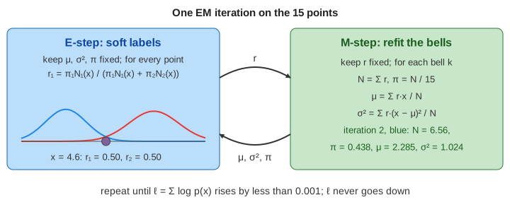
With the parameters fixed, the E-step asks of every point: how much of it does each bell explain? The responsibility of bell k for point x is its weighted height at x, divided by the total height:
So r₁ + r₂ = 1 for every point. The page walks through the point x = 4.6, which sits between the two groups. From the good start (μ = 1 and 9, σ² = 1) it is much closer to blue, so r₁ = 0.961 (Demo 1: one E-step). One iteration later both bells have moved and widened, and the same point is split almost evenly, r₁ = 0.498 (Demo 2). The parameters do not change in an E-step.
The M-step: weighted mean, variance and weight
With the responsibilities fixed, the M-step refits each bell as if r were the share of each point that belongs to it. These are the usual formulas for a mean and a variance, with every point weighted by r:
| number | formula | iteration 2, blue |
|---|---|---|
| soft count Nk | Σ rk | 6.56 of the 15 points |
| weight πk | Nk / 15 | 0.438 |
| mean μk | Σ rk·x / Nk | 2.285 |
| variance σk² | Σ rk·(x − μk)² / Nk | 1.024 |
A point with r = 0.5 counts as half a point for each bell. If every r were 0 or 1, these would be the plain mean and variance of each group. A variance is never allowed below 0.01, so a bell cannot shrink onto a single point.
The log-likelihood never goes down
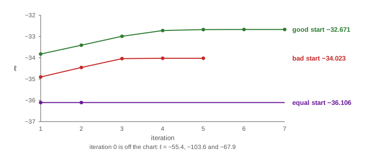
The score EM improves is the log-likelihood ℓ = Σ log p(x), summed over the 15 points, where p(x) = π₁N₁(x) + π₂N₂(x) is the grey curve. A higher ℓ means the mixture puts more density where the points are. Each E-step + M-step pair can only raise ℓ or keep it: the E-step builds a lower bound on ℓ that touches it at the current parameters, and the M-step climbs that bound. From the good start (Demo 3):
| iteration | μ₁ / μ₂ | σ₁² / σ₂² | π₁ / π₂ | ℓ |
|---|---|---|---|---|
| 0 | 1 / 9 | 1 / 1 | 0.5 / 0.5 | −55.426 |
| 1 | 2.419 / 7.196 | 1.229 / 1.805 | 0.467 / 0.533 | −33.824 |
| 2 | 2.285 / 7.054 | 1.024 / 2.082 | 0.438 / 0.562 | −33.410 |
| 3 | 2.161 / 6.963 | 0.749 / 2.234 | 0.416 / 0.584 | −32.989 |
| 7 | 2.029 / 6.841 | 0.468 / 2.499 | 0.390 / 0.610 | −32.671 |
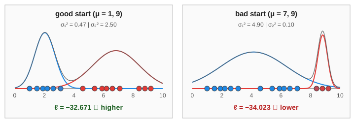
The gains shrink fast: +21.6, then +0.41, and after iteration 7 less than 0.001, so EM stops. Blue ends on the left group 1.0–3.1, red on the rest 4.6–9.2. The value of ℓ is negative because a density below 1 has a negative log; only differences between ℓ values matter.
A bad start ends at a worse fit
"ℓ never goes down" only promises a climb to the nearest hilltop, a local optimum. Start both bells on the right, at μ = 7 and 9 (Demo 4). Red catches the three far points 8.4, 8.8 and 9.2 and shrinks to σ² = 0.10, while blue stretches over the other twelve (σ² = 4.90). EM converges in 5 iterations to ℓ = −34.023, lower than −32.671, and stays there: every later step only climbs, and this hill has no way up.
A third start shows a trap of another kind. If both bells start equal (μ = 5 and 5, Demo 5), every point gives each bell r = 0.5. The M-step then fits both to all the data in the same way, so they stay equal forever: one wide bell (μ = 4.97, σ² = 7.22) counted twice, ℓ = −36.106. This is a fixed point of EM but not a hilltop: any small difference between the two bells would grow, which is why real code never starts two bells at the same place.
The usual fix is to run EM from several starts, often from k-means results, and keep the run with the
highest ℓ (n_init in scikit-learn). For how a mixture differs from k-means on 2D data, with
ellipses and the hard vs soft assignment, see k-means vs Gaussian Mixture. For
the k-means loop itself, see K-Means Clustering.
EM in general
The mixture is one case of a general recipe for models with hidden variables, here the unknown group z of each point. The E-step computes how likely each value of z is, given the data and the current parameters. The M-step picks the parameters that maximise the expected log-likelihood under those probabilities, the quantity usually called Q(θ | θold). The same pattern trains hidden Markov models (the Baum–Welch algorithm) and fills in missing values in data.
| E-step | M-step | |
|---|---|---|
| keeps fixed | μ, σ², π | the responsibilities r |
| computes | r for every point and bell | N, μ, σ², π for every bell |
| on the canvas | point colours, the r table | the bells move, a new ℓ dot |
See also K-Medoids and the Silhouette Score for hard clustering with real points as centres, and choosing the number of clusters by the average silhouette.
What the page leaves out
The page uses one dimension and exactly two bells. Real data has many dimensions, where each bell has a covariance matrix; the 2D case is on the k-means vs GMM page. How to choose the number of bells (BIC, AIC, silhouette) is left out. It also skips the proof of the lower bound (Jensen's inequality), random and k-means++ starts, and variants such as hard EM, online EM and the Bayesian mixture with a prior on the weights.