Value Iteration on a Grid World

The idea: plan on a slippery floor

A robot lives on a 4×3 grid. Reaching the goal (4,3) is worth +1, falling into the pit (4,2) costs −1, and both end the game. (2,2) is a wall. The floor is slippery: a move goes where it is aimed with probability 0.8, and slides to the left or the right of that with probability 0.1 each. Bumping into the wall or the edge means staying put. Every move also earns a small living reward r, by default −0.04, so wandering around costs a little.

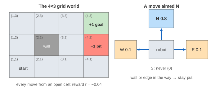
The question is not "what is the shortest path" but "what should I do in each cell, given that I might slip". Value iteration answers it by computing a value V(s) for every cell, the reward the robot can expect from there if it plays well, and then reading the best move off the values. Pick a demo and press Run Demo, or use Bellman Update, Sweep and Run to Convergence yourself.

A Markov decision process

The grid is a Markov decision process (MDP): a set of states s (the 9 open cells), actions a (N, E, S, W), transition probabilities P(s'|s,a) (0.8 / 0.1 / 0.1), a reward r for each move and a discount γ between 0 and 1 that makes a reward one step later worth γ times as much. "Markov" means the next state depends only on the current state and action, not on how the robot got there.

The Bellman update

For one cell, try each of the four actions. For each action, list where the robot can end up, weight each neighbour's value by its probability, and add the reward:

Q(s,a) = Σ P(s'|s,a) · [ r + γ · V(s') ]  =  r + γ · Σ P(s'|s,a) · V(s')
V(s)  ←  max over a of Q(s,a)

Q(s,a) is the action value: what the action is worth if the robot plays well afterwards. The new V(s) is the best of the four. At the start every value is 0, so for (3,3) next to the goal: E gives 0.8·1 + 0.1·0 + 0.1·0 = 0.8 and Q = −0.04 + 0.8 = 0.76; N and S each slip into the goal only 10% of the time (Q = 0.06); W gives −0.04. The new value is 0.76 (Demo 1). Next to the pit the sums mix good and bad news: from (3,2), N risks a 0.1 slide into the pit (Demo 2).

Sweeps and convergence

A sweep applies the Bellman update to every cell. The textbook version is synchronous: sweep k+1 reads only the old values V_k and writes V_k+1, so the order of the cells does not matter. After sweep 1 only the cells next to a terminal know about it; after sweep 2 their neighbours do; the values spread outward from the goal one cell per sweep (Demo 3).

Each sweep changes the values less than the one before. The page stops when the largest change in a sweep, Δ, is below ε = 0.001. With r = −0.04 and γ = 1 that takes 19 sweeps, and the values match the ones printed in Russell and Norvig: V(1,1) = 0.705, V(3,3) = 0.918, V(4,1) = 0.387 (the book prints 0.388, the exact limit). The chart on the right shows Δ on a log scale: it falls by a roughly constant factor per sweep. With γ < 1 that is guaranteed: the Bellman update is a contraction, and each sweep shrinks the error by at least a factor γ.

Policy extraction

The values are not the answer yet. The policy π(s) is the action with the largest Q(s,a) under the converged values: one arrow per cell (Extract Policy).

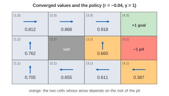
Two cells are interesting. (3,2), right next to the pit, goes N and accepts a 10% chance of slipping into the pit, because the long way round costs more. (4,1) goes W, away from the pit, instead of N along it. With deterministic moves (Demo 4) both risks disappear: every cell takes a shortest path, 6 sweeps suffice, and V(1,1) = 1 − 5 × 0.04 = 0.80.

How the living reward changes the policy

The reward per move decides how much the robot hurries.

r	(3,2) next to the pit	(4,1) under the pit	sweeps
−2 (Demo 5)	E: straight into the pit	N: straight into the pit too	15
−0.4	N: shortest way, risky	W	12
−0.04 (default)	N	W: the long way	19
−0.01 (Demo 6)	W: faces the wall, never slips into the pit	S: faces the edge, slips only sideways	45
+0.1 (Demo 7)	every arrow avoids both exits: living is worth more than leaving		never

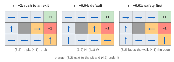
With a very negative r, every move hurts more than the pit does, so cells near the pit jump in (Demo 5). With a slightly negative r, moves are cheap and the pit is the only real danger: (3,2) faces the wall, so a move either bumps (stays) or slips N or S, never E into the pit; (4,1) faces the bottom edge for the same reason (Demo 6). With a positive r and γ = 1, every extra move adds reward, so the best plan is never to finish; the values grow by 0.1 per sweep forever and value iteration never converges (Demo 7).

γ: how far ahead the robot looks

The discount γ makes a reward t steps away worth γ^t today. With γ = 1 the +1 counts in full however far away it is. With γ = 0.5 (Demo 8), the goal four steps away is worth only 0.5⁴ ≈ 0.06, so far cells barely feel it: V(1,1) = −0.062, most of it the cost of living. A small γ also makes value iteration converge faster (7 sweeps), because the error shrinks by at least a factor γ per sweep. γ < 1 is what guarantees convergence when episodes could go on forever.

Policy iteration

Policy iteration works on the arrows directly. Start with any policy (here: every arrow E). Evaluate it: with the arrows fixed there is no max, just V(s) = r + γ Σ P V(s') for the one chosen action. Improve it: point each arrow at the best Q under those values. Repeat until no arrow changes (Demo 9). Here it needs 4 rounds, but each evaluation is itself a full solve. Both methods end with the same policy. Value iteration is the special case that improves after a single evaluation sweep.

From planning to learning

Value iteration needs the model: it reads P(s'|s,a) and r directly. A real robot often does not know them. Q-Learning learns the same Q values from experience instead, by trying moves and averaging what happens, and ends with the same kind of arrows. The update has the same shape: r + γ · (best value of the next state).

See also Dijkstra's algorithm and Bellman-Ford, which solve the deterministic version of the same equation (shortest paths) and also relax distances until nothing changes, and dynamic programming, of which value iteration is an example. Monte Carlo Tree Search plans by sampling instead of sweeping every state.

An MDP is a Markov chain with actions and rewards; the plain chain is in Markov Chains and Random Walks.

What the page leaves out

In-place (Gauss-Seidel) and asynchronous updates, which use new values within the same sweep and usually converge faster; prioritized sweeping; the bound ε(1−γ)/γ that turns Δ into a guarantee on the policy's loss; rewards that depend on the action or the next state; large or continuous state spaces, where values are approximated by a function (fitted value iteration, deep RL); partially observable MDPs, where the robot does not know which cell it is in; and solving policy evaluation exactly as a linear system.

References

Russell & Norvig: Artificial Intelligence, A Modern Approach (chapter 17, Making Complex Decisions)

Sutton & Barto: Reinforcement Learning, An Introduction (chapter 4, Dynamic Programming)

UC Berkeley CS188: Markov Decision Processes