The idea: learn what each move is worth, by trying
An agent walks in a 4 × 4 grid. It starts at S in the bottom-left corner. The top-right cell pays +1 and ends the episode; the cell under it is a pit that pays −1. One cell is a wall. Every other move pays 0. The agent does not know the map or the rewards. It only sees where it is, what it did, and what it got.
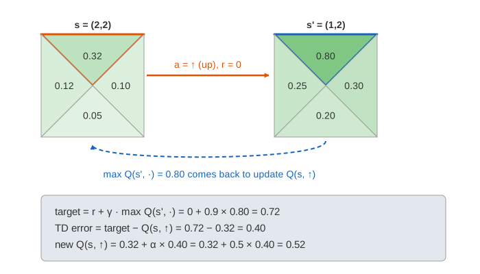
Q-learning keeps a table Q(s, a): for every cell s and every action a (↑ → ↓ ←), a guess of the total reward it will get if it takes a in s and plays well afterwards. On the canvas these are the 4 small boxes in each cell, green when positive and red when negative. The arrow in a cell points to the box with the largest number: the greedy action. All guesses start at 0, and the arrows appear as the agent learns.
One step: choose, act, update
Every move has three parts (Demo 1: one step, the update rule, or press Step):
- Choose an action with ε-greedy (next section).
- Act: move, land in the next cell s', receive the reward r.
- Update the one box for (s, a):
Q(s,a) ← Q(s,a) + α · [ r + γ · max Q(s',·) − Q(s,a) ]| part | meaning |
|---|---|
r + γ · max Q(s',·) | the target: the reward just received plus the best the agent thinks it can do from s', discounted by γ. For a terminal s' the max is 0. |
target − Q(s,a) | the TD error (temporal difference): how wrong the old guess was. |
α | the learning rate: how far the guess moves toward the target, from 0 (not at all) to 1 (all the way). |
γ | the discount factor: a reward k moves later counts γk as much as one now. |
The rule uses the best action in s', not the action the agent will actually take there. That is what makes Q-learning learn the greedy policy even while it explores.
How the reward spreads backwards
At first every target is 0 + γ × 0 = 0, so most updates change nothing. Only the move that enters the +1 gets a target that is not 0. In episode 1, only the last move learns (Demo 2). In episode 2, the move before it sees a positive max Q(s', ·) and learns too. Each episode carries the value one more move back.
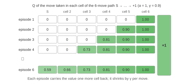
With α = 0.5 the numbers grow more slowly, but they end at the same place: the cell k moves from the goal is worth 0.9k−1. S is 6 moves from the +1, so after enough episodes max Q(S, ·) = 0.95 = 0.59. The chart on the canvas shows max Q(S, ·) after each episode. In Demo 3: 50 episodes it climbs to 0.59 after about 22 episodes, and the arrows form a shortest path from S to the +1, around the pit.
ε-greedy: explore or exploit
Before each move the agent draws a random number u between 0 and 1. If u < ε it explores: it takes a random action. Otherwise it exploits: it takes the action with the largest Q (ties are broken at random). The status panel shows which one happened. Exploiting collects the reward it already knows about; exploring is the only way to find a better one.
The world select adds a third exit at (3,3) that pays only +0.3, 3 moves from S. With ε = 0 the agent finds that exit first, by chance, and from then on always goes back to it: the +1 is 6 moves away and it never walks there to find out (Demo 4). max Q(S, ·) stops at 0.24 = 0.9² × 0.3. With ε = 0.8 the agent wanders a lot, finds the +1, and its greedy path switches to it: max Q(S, ·) = 0.59 (Demo 5). It behaves randomly 80 % of the time and still learns the best route. Q-learning is off-policy: what it learns does not depend on how it explores, as long as it keeps trying every action. In practice ε starts high and is lowered over time.
γ: short-sighted or far-sighted
γ decides how much the future counts. With the +0.3 exit 3 moves away and the +1 6 moves away:
| γ | Q(S, toward +1) = γ5 × 1 | Q(S, toward +0.3) = γ2 × 0.3 | greedy choice |
|---|---|---|---|
| 0.9 | 0.59 | 0.24 | +1, the long way (Demo 5) |
| 0.5 | 0.03 | 0.075 | +0.3, the quick exit (Demo 6) |
In Demo 6 the agent has found the +1 (Q(S, ↑) is 0.03, not 0), but with γ = 0.5 a reward 6 moves away is worth too little. It takes the +0.3 on purpose. This is not a bug: γ is part of the problem statement. A low γ suits tasks where only the near future matters or the future is uncertain; a γ close to 1 makes the agent patient.
α: how much one sample counts
With deterministic moves every sample of a move is the same, and α = 1 is fine. With slippery moves (80 % as intended, 10 % to each side) the same move gives different results. α = 1 overwrites Q with the latest sample, so the values jump: after a lucky run max Q(S, ·) is 0.59, after a slide toward the pit it drops to 0.2 or less (Demo 7, see the chart). α = 0.1 moves only 10 % toward each sample, which averages the luck out: the chart rises slowly and smoothly (Demo 8). The same trade-off as the learning rate in Gradient Descent: too large jumps around, too small takes forever. Convergence proofs need α to shrink over time.
Q-learning vs value iteration
Value Iteration solves the same kind of grid when the model is known: it uses the move probabilities and rewards to update every cell in sweeps with the Bellman equation. Q-learning has no model. It learns the same values from samples, one move at a time, only where the agent has actually been. That is why it needs many episodes and exploration, and why it is called model-free.
| value iteration | Q-learning | |
|---|---|---|
| needs the model (P, R) | yes | no, it samples |
| updates | every state, each sweep | one (s, a) per move |
| stores | V(s) | Q(s, a), so the policy is just argmax |
| exploration | not needed | needed (ε-greedy) |
See also Monte Carlo Tree Search, which also learns move values from playouts, and Grid Pathfinding, which finds the shortest path when the map is known.
See also Supervised vs Unsupervised vs Reinforcement Learning, which compares the one-step form of RL with supervised and unsupervised learning on the same data.
The same reward-driven loop trains chat models in RLHF, where a learned reward model plays the environment; see RLHF vs DPO.
What the page leaves out
A step cost (a small negative reward per move), decaying ε and α over time, optimistic initial values, SARSA (the on-policy twin that uses the action actually taken next), Double Q-learning (against the overestimation that max causes), eligibility traces, experience replay, and deep Q-networks (DQN), which replace the table with a neural network so the states can be images.