Simulated Annealing Visualization | Hill Climbing vs Cooling

The idea: search by small moves on a landscape

Local search keeps one current state and tries to improve it by small changes. Each state x has a score f(x); the goal is the x with the highest score. The states next to x are its neighbours. Here x runs from 0 to 29 and the neighbours of x are x−3 … x+3. Local search needs no tree and almost no memory, so it works on problems far too big to search in full: timetables, chip layouts, travelling-salesman tours.

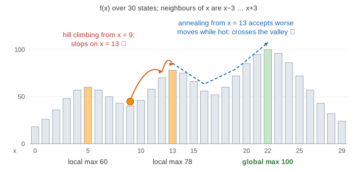
The landscape on the canvas has three peaks: local maxima at x = 5 (f 60) and x = 13 (f 78), and the global maximum at x = 22 (f 100). The orange ball is the current state.

Hill climbing

Hill climbing (steepest ascent) looks at every neighbour and moves to the best one, but only if it is higher. When no neighbour is higher, it stops. That point is a local maximum, and it may not be the global one: from x = 13 every way to x = 22 first goes down to f = 52 at x = 17. (Demo 1: hill climbing gets stuck: from x = 9 it moves to 12, then 13, and stops at f = 78.)

x = start
loop:
    x' = the best neighbour of x
    if f(x') <= f(x): return x        # local maximum
    x = x'

Other traps of the same kind: a plateau (all neighbours equal, no direction to go) and a ridge (higher ground exists, but not one neighbour step away).

Random restarts

Random-restart hill climbing climbs again from a random state each time it gets stuck and keeps the best top. Every start belongs to one basin: here x = 0–8 climb to 5, x = 9–16 to 13, and x = 17–29 to 22. A random start lands in the global basin with chance 13/30, so 4 random restarts miss it with chance (17/30)⁴ ≈ 10%. (Demo 2: random restart finds the global max: tops 13, 13, 5, 22, 5; the best is 22.)

Simulated annealing

Simulated annealing picks one random neighbour x′ and computes Δ = f(x′) − f(x). A better or equal move (Δ ≥ 0) is always taken. A worse move is taken with probability

P = e^{Δ / T}

where T is the temperature. The page draws a random r in [0, 1) and accepts when r < P (the Metropolis rule). A green ✓ ring marks a move taken, a red ✗ ring a move refused.

Δ (how much worse)	T = 40	T = 10	T = 3	T = 1
−5	0.88	0.61	0.19	0.01
−10	0.78	0.37	0.04	≈ 0
−20	0.61	0.14	≈ 0	≈ 0
−40	0.37	0.02	≈ 0	≈ 0

Hot, the ball wanders almost freely; cold, it only goes uphill, like hill climbing. Small losses pass more often than big ones at every temperature. (Demo 5: acceptance probability vs temperature walks the table column by column.) The name comes from metallurgy: metal cooled slowly settles into a low-energy crystal, cooled fast it freezes in a worse state.

The cooling schedule

The page uses geometric cooling: T starts at T₀ = 40 and after every iteration T ← α·T, for 60 iterations.

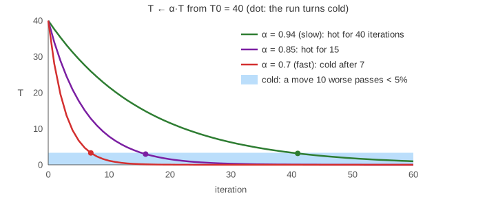
Temperature against iteration for alpha 0.94, 0.85 and 0.7, all starting at 40. A shaded band near the bottom marks the cold zone where a move 10 worse passes less than 5 percent of the time; alpha 0.7 enters it at iteration 7, alpha 0.85 at 16, alpha 0.94 at 41. — With α = 0.7 the run is cold after 7 iterations, too soon to cross a valley; with α = 0.94 it stays hot for 40.

Starting from the local maximum x = 13 with seed 2, α = 0.94 crosses the valley and ends on x = 22 (Demo 3: annealing escapes the local max). With the same seed and α = 0.7 the temperature collapses before the ball gets out, and it ends where it started, on x = 13 (Demo 4: cooling too fast = hill climbing).

Other schedules: linear (T ← T − c), logarithmic (T = c / log(1 + k), slow enough for a convergence proof but far too slow in practice), and reheating when the search stalls.

How often each method wins here

Measured over seeds 1–100 on this landscape (the page's own code):

Method	Start	Ends on x = 22
Hill climbing	x = 9 or 13	never
Random restart, 5 climbs	x = 9	88 of 100
Annealing, α = 0.94	x = 13	46 of 100
Annealing, α = 0.85	x = 13	24 of 100
Annealing, α = 0.7	x = 13	13 of 100

On a 30-state line random restarts win: 5 random starts cover the landscape well. Annealing pays off when the space is huge and the good basins are tiny, so random starts almost never land in one, but a walk that may go downhill can follow the landscape towards them. Annealing is a heuristic: it does not promise the global maximum, and slower cooling only makes it more likely.

See also Gradient Descent (the same "follow the slope" idea on a continuous loss, with the same trouble with local minima), Genetic Algorithm (a population instead of one ball), and A* Search (systematic search that keeps a frontier instead of one state).

See Monte Carlo Estimation of π for how seeded random sampling estimates a number, and why 100× more samples buy one more digit.

See Travelling Salesman Heuristics for 2-opt on a real tour: swapping two edges untangles crossings until the tour is stuck on a local optimum.

What the page leaves out

Real problems have huge, many-dimensional state spaces (a tour of 1000 cities, a timetable), so a neighbour is a small edit such as swapping two cities (2-opt), and f is usually a cost to minimize, which flips the sign of Δ. Real runs use thousands of iterations per temperature, choose T₀ from the typical size of Δ, stop when nothing changes, and return the best state seen rather than the last one. Variants such as tabu search, parallel tempering and stochastic hill climbing are not shown.