The idea: every matrix is rotate, stretch, rotate
Apply a 2×2 matrix A to the unit circle and you always get an ellipse (or a segment, if A squashes the plane flat). The singular value decomposition says why: any A can be written as A = U·Σ·Vᵀ, three simple moves in a row.
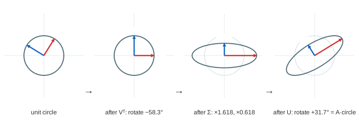
- Vᵀ rotates the plane so two special perpendicular unit vectors, v1 and v2, land on the x and y axes.
- Σ = [[σ1, 0], [0, σ2]] stretches x by σ1 and y by σ2. These singular values are never negative, and σ1 ≥ σ2.
- U rotates the stretched axes onto two perpendicular unit vectors u1 and u2.
So A·v1 = σ1·u1 and A·v2 = σ2·u2: the ellipse's semi-axes have lengths σ1 and σ2, and σ1·σ2 = |det A| is the factor by which A scales area (see Determinant). (Demo: SVD of a shear.)
Computing the SVD of a 2×2
The v's come from the symmetric matrix AᵀA: its eigenvectors are v1 and v2 and its eigenvalues are σ1² and σ2². Then σi = ‖A·vi‖ and ui = A·vi / σi. For the shear, AᵀA = [[1, 1], [1, 2]] has eigenvalues 2.618 and 0.382, so σ1 = 1.618 and σ2 = 0.618.
| Matrix | Eigenvalues | Singular values | Rotations |
|---|---|---|---|
| Shear [[1, 1], [0, 1]] | 1, 1 | 1.618, 0.618 | −58.3°, then +31.7° |
| Symmetric [[2, 1], [1, 2]] | 3, 1 | 3, 1 | −45°, then +45° (U = V) |
| Scaled rotation [[1, −1], [1, 1]] | 1 ± i | 1.414, 1.414 | none, then +45° |
For a symmetric matrix with positive eigenvalues, U = V and the singular values are the eigenvalues (Demo: SVD of a symmetric matrix). For other matrices they differ: the shear keeps only one direction (eigenvalue 1, twice), yet it still stretches some direction by 1.618. Singular values exist for every matrix, even non-square ones; eigenvalues may not. Compare Eigenvectors and Linear Transformations.
From SVD to PCA
Principal component analysis asks: in which direction does a cloud of points spread the most? The page does it in four steps.
- Centre: subtract the mean from every point, so the cloud sits around the origin.
- Covariance: C = Σ x·xᵀ / (n − 1) = [[var x, cov(x, y)], [cov(x, y), var y]].
- Eigenvectors of C: v1 (PC1) is the direction of largest variance λ1, v2 (PC2) is perpendicular to it with variance λ2. C is symmetric, so they are always perpendicular.
- Variance explained: PC1 carries λ1 / (λ1 + λ2) of the total variance.
The arrows are drawn 2·√λ long, two standard deviations along each axis. The link to SVD: if X is the n×2 matrix of centred points, then C = XᵀX / (n − 1), so the principal axes are exactly the v's of the SVD of X, and λi = σi² / (n − 1). Libraries compute PCA with an SVD for this reason. (Demo: PCA on a correlated cloud: C = [[0.95, 0.44], [0.44, 0.33]], λ1 = 1.18, λ2 = 0.10.)
Projection and variance explained
To reduce 2D data to 1D, replace each point p by one number, its score t = p·v1, and draw it at t·v1 on the PC1 line. The spread of the scores is λ1 (the part kept); the squared distances to the line add up to λ2·(n − 1) (the part lost). No other line keeps more variance or loses less squared distance.
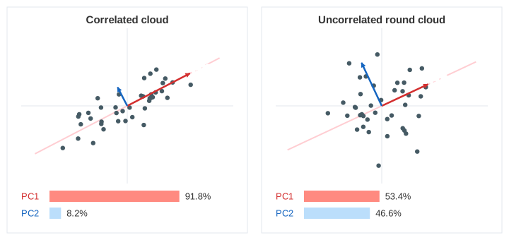
On the correlated cloud PC1 explains 91.8%, so one number per point loses little (Demo: projection to 1D). On an uncorrelated round cloud no direction is special: PC1 explains only 53.4% and the projection throws away almost half (Demo: uncorrelated cloud). The same idea fits a line by perpendicular distance, unlike least squares, which measures vertical distance.
Where SVD and PCA are used
- Dimensionality reduction: keep the top k components before clustering (k-means) or plotting.
- Compression: keep the largest σ's of an image or a matrix (low-rank approximation).
- Recommenders and search: latent factors and latent semantic analysis are truncated SVDs.
- Numerics: σ1 / σ2 is the condition number; the pseudo-inverse comes from the SVD.
See also Eigenvectors, Linear Transformations, Matrix Multiplication and K-Means Clustering.
See also PCA vs t-SNE: the same projection next to a non-linear neighbour embedding, and the data where PCA puts groups on top of each other.
What the page leaves out
Only 2×2 matrices with positive determinant (a negative determinant adds a reflection to U) and 2D data. Non-square and rank-deficient matrices, how SVD is computed in practice (Golub–Kahan bidiagonalisation), scaling features before PCA, choosing how many components to keep, and non-linear methods such as kernel PCA and t-SNE.