The idea: the determinant is an area factor
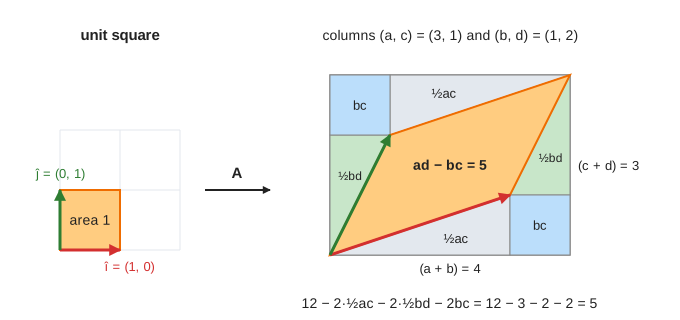
A 2×2 matrix A = [a b; c d] is a linear map of the plane. It sends the basis vector î = (1, 0) to its first column (a, c) and ĵ = (0, 1) to its second column (b, d). Every other point follows: (x, y) goes to x·(a, c) + y·(b, d). So the grid of unit squares becomes a grid of copies of one parallelogram, the one spanned by the two columns. Its signed area is the determinant:
On the canvas, the faint grid stays put and is the ruler: each faint square has area 1. The blue grid, the orange hatched square and the purple F move with the matrix. The red arrow is where î lands, the green one where ĵ lands.
Why ad − bc, in two steps
The page moves the columns one at a time. First only î moves, to (a, c), with ĵ still at (0, 1): that is the matrix [a 0; c 1]. The square becomes a parallelogram whose two vertical sides have length 1 and stand a apart, so its area is a. Then ĵ moves from (0, 1) to (b, d). Split (b, d) into a part along the first column, (b/a)·(a, c), and what is left, (0, d − bc/a). Sliding a side along the other one is a shear and keeps the area, so only the leftover height counts: a · (d − bc/a) = ad − bc.
Every area scales by the same factor
The map is linear, so every grid cell turns into the same parallelogram. Any shape can be filled with tiny squares, and each tiny square’s area is multiplied by |det A|, so the whole shape’s area is too. With A = [2 0; 0 3] the unit square becomes a 2 × 3 rectangle that covers exactly 6 faint squares (Demo: scaling, det 6).
| Matrix | A | det | What happens |
|---|---|---|---|
| shear | [1 1; 0 1] | 1 | the square leans over; area 1 kept |
| rotate 90° | [0 −1; 1 0] | 1 | turned, same size |
| scale | [2 0; 0 3] | 6 | every area ×6 |
| mixed | [2 1; −1 1] | 3 | stretched and slanted, area ×3 |
| reflection | [−1 0; 0 1] | −1 | mirror in the y-axis; area kept, orientation flipped |
| singular | [2 1; 2 1] | 0 | everything lands on the line y = x |
det = 1: shapes change, areas do not
A shear [1 1; 0 1] keeps î and slides ĵ to (1, 1). The square leans into a parallelogram with the same base and the same height, so its area stays 1 (Demo: shear, det 1). Rotations also have det 1. Shears are exactly what Gaussian elimination uses when it adds a multiple of one row to another, which is why that step never changes the determinant.
Negative det: orientation flips
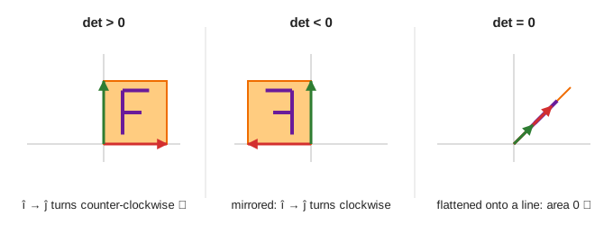
The sign of ad − bc says whether the map keeps orientation. With det > 0, turning from the red arrow to the green one is still counter-clockwise, as it is from î to ĵ. With det < 0 it is clockwise: the plane has been flipped over like a page, and the F comes out mirrored (Demo: reflection, det −1). Area is scaled by |det|; the sign carries the flip.
det = 0: the plane collapses
When the two columns are parallel, as (2, 2) and (1, 1) are, the parallelogram is flat. Every point of the plane lands on one line, so every area becomes 0 (Demo: singular, det 0). Different points land on the same spot, so nothing can undo the map: a matrix has an inverse exactly when det ≠ 0. For a system Ax = b this means either no solution or infinitely many.
det(AB) = det A · det B
Applying B and then A is one map, the product AB. B scales every area by det B, then A scales the result by det A, so
Press Then apply to put a second matrix on top of the current one. Reflect, then scale: AB = [2 0; 0 3]·[−1 0; 0 1] = [−2 0; 0 3], and ad − bc = −6 = 6 · (−1) (Demo: det(AB) = det A · det B). The signs multiply too: two reflections cancel and give det > 0 again. Consequences: det(A−1) = 1 / det A, and if any factor is singular the product is.
Computing it for bigger matrices
For an n×n matrix the determinant is the signed volume of the box spanned by the columns. Nobody uses the cofactor formula beyond 3×3: it has n! terms. Instead, row-reduce to an upper triangular matrix. Adding a multiple of a row (a shear) leaves det alone, swapping two rows flips its sign, and the determinant of a triangular matrix is the product of its diagonal. That is O(n³) work. The eigenvalues multiply to the determinant too.
See also Rotation and Scaling in 2D (matrices applied to a shape), Eigenvectors (directions a matrix only stretches) and Gaussian Elimination (row reduction, where det appears as the product of the pivots).
See also Matrix Multiplication (how the product AB is computed, and why it means apply B, then A). See Linear Transformations for where î and ĵ land, change of basis, and why det = 0 means no inverse (the null space).
What the page leaves out
Only 2×2 matrices with small whole-number entries are drawn, so the grid stays inside the panel. The 3×3 case (signed volume of a parallelepiped, the triple product), the cofactor and Leibniz formulas, Cramer’s rule, the Jacobian determinant in a change of variables, and floating-point issues (a determinant near 0 does not mean a matrix is nearly singular) are not shown.