The idea: many small trees, combined in two different ways
A single decision tree is easy to train and easy to read, but it is unstable: change a few training rows and you get a different tree. Ensembles train many trees and combine them. The two most used ones combine them in opposite ways.
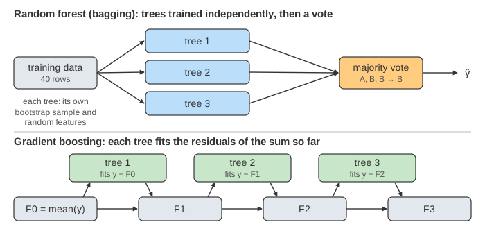
- A random forest (bagging) trains its trees independently, each on a slightly different copy of the data, and lets them vote.
- Gradient boosting trains its trees one after another. Each new tree is fitted to the errors the trees before it still make, and is added to them.
Pick a method in the Method menu. Next Tree builds one tree step by step, Train All builds the rest quickly, and Predict ? shows how the trained ensemble answers. All data is generated from fixed seeds, so every run gives the same numbers.
Random forest, step 1: a bootstrap sample per tree
The forest panel has 40 points with two features x1, x2. Class B (orange) is the side above the line x1 + x2 = 10, class A (blue) the side below it, and 3 labels are flipped to act as noise.
Every tree gets its own bootstrap sample: 40 draws with replacement from the 40 rows. Some rows are drawn two or three times (the number in a dot), and about 1/e ≈ 37% are never drawn. Those are the tree's out-of-bag (OOB) rows, shown faded. Each tree therefore learns from a slightly different data set. (Demo: inside one tree)
Step 2: a random feature at every split
Bootstrap samples alone would still give similar trees: they would all split first on the strongest
feature. So at every node a forest only looks at a random subset of the features
(max_features). With two features the page uses max_features = 1: each node draws
x1 or x2 at random and finds the best threshold on that feature, the one that lowers the
Gini impurity most. If the drawn feature cannot split the node, the other one is tried, as
scikit-learn does. The trees grow to max_depth = 3.
The result is five quite different trees. On 400 fresh points (labelled by the true rule) they score 77%, 69%, 72%, 76% and 74%.
Step 3: majority vote
To classify a point, every tree answers on its own and the forest returns the class with the most votes. On the main plot, a darker tint means more trees agree. The individual mistakes of the trees are different, so many of them cancel out in the vote:
| n_estimators | Test accuracy |
|---|---|
| 1 tree (tree 1) | 77% |
| 3 trees | 80% |
| 5 trees | 92% |
| average single tree | 74% |
(Demo: 1 tree vs a forest of 5) For the query point ? = (8.0, 3.5), whose true class is B, tree 1 says A, but trees 2, 3 and 4 say B: the forest answers B, 3 to 2. (Demo: the forest votes on a new point)
Gradient boosting: fit the residuals, one tree at a time
The boosting panel is a regression problem: 20 points scattered around the grey curve y = 2 + 1.5·sin(0.8x). The model starts as a single number, F0 = the mean of y. Then each round m:
- compute the residuals ri = yi − Fm−1(xi) (the red stems, and the orange dots in the lower plot);
- fit a small tree hm to the residuals. Here it is a stump (one split): the threshold with the least squared error, each leaf predicting its mean residual (green line);
- shrink it by the learning rate ν and add it: Fm(x) = Fm−1(x) + ν·hm(x).
For squared error the residual is exactly the negative gradient of the loss with respect to F(x), which is where the name comes from: each tree is one step of gradient descent, taken in the space of functions. (Demo: boosting, 3 trees on the residuals)
The learning rate and overfitting
Training error can only go down, tree after tree. Test error (200 fresh points) is what matters:
| ν | Train MSE after 20 trees | Best test MSE | Test MSE after 20 trees |
|---|---|---|---|
| 0.1 | 0.74 | 0.47 (still falling) | 0.47 |
| 0.3 | 0.22 | 0.25 at 19 trees | 0.27 |
| 1.0 | 0.10 | 0.27 at 3 trees | 0.39 |
With ν = 1 the first few trees fix most of the error, and the later ones start fitting the noise of single points: training error falls while test error rises (Demo: ν = 1.0 overfits). With ν = 0.1 the steps are so small that 20 trees are not enough (Demo: ν = 0.1 learns slowly). In practice one takes a small ν and many trees, and stops when a validation score stops improving (early stopping).
Bias vs variance
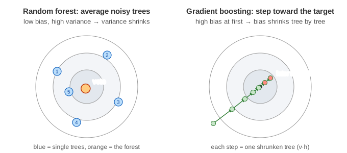
The error of a model on new data has two parts that can be reduced. Bias is the error of being too simple: the average model misses the truth. Variance is the error of being too sensitive: a different training set gives a very different model.
| Random forest | Gradient boosting | |
|---|---|---|
| Trees trained | independently, in parallel | one after another |
| Each tree sees | a bootstrap sample, random features | all rows, the current residuals |
| Typical tree | deep (low bias, high variance) | shallow, 1–6 levels (high bias, low variance) |
| Combined by | vote / average | sum, each tree shrunk by ν |
| Mainly reduces | variance | bias |
| More trees | never hurts, only costs time | can overfit: needs early stopping |
| Tuning | works well with defaults | ν, number of trees and depth matter |
See also Decision Tree Learning for how one tree picks its splits, Linear Regression for the squared-error loss used here, k-Nearest Neighbors and Naive Bayes for other classic classifiers.
What the page leaves out
Real forests use hundreds of fully grown trees and average class probabilities rather than counting votes; the page uses 5 trees of depth 3. Thresholds are restricted to a 0.5 grid (like the histogram bins of LightGBM or HistGradientBoosting). Boosting is shown for regression with squared error and stumps; classification boosting fits the gradient of the log-loss, and XGBoost, LightGBM and CatBoost add second-order steps, regularization, row and column subsampling and leaf-wise growth. Out-of-bag error estimates, feature importance, extra-trees and AdaBoost are only mentioned here.