Naive Bayes Spam Filter

The idea: which class makes these words most likely?

A Naive Bayes spam filter learns from emails that are already labelled spam or ham (not spam). For a new email it asks, for each class: how likely is this class at all, and how likely are these words if the email belongs to it? The class with the larger product wins.

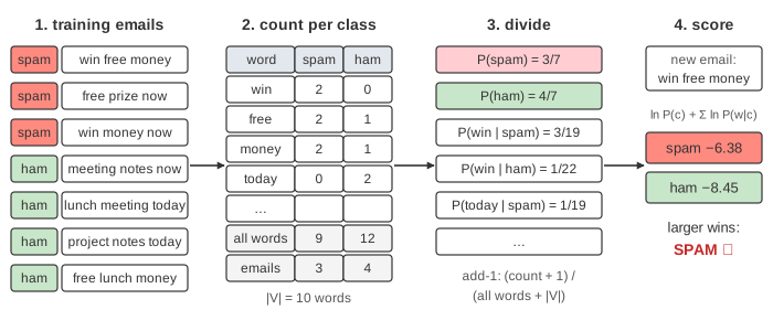
Bayes' rule says P(spam | email) ∝ P(spam) × P(email | spam). The hard part is P(email | spam): no two emails are the same. The naive assumption cuts it into one factor per word, as if the words were chosen independently once the class is known:

P(spam | w1 w2 … wn)  ∝  P(spam) × P(w1 | spam) × P(w2 | spam) × … × P(wn | spam)

The assumption is false (“free” and “money” go together), but the filter only needs the right winner, not the right probability, and it gets that surprisingly often.

Training is counting

The page trains on 7 short emails: 3 spam, 4 ham. Each email adds 1 to its class's email count and 1 to every one of its words in its class's column (Demo 1). Then two divisions give the whole model:

• Prior P(c) = emails in class c / all emails: P(spam) = 3/7, P(ham) = 4/7.
• Likelihood P(w | c) = how often word w appears in class c / all words in class c. Spam has 9 words, “win” is 2 of them, so P(win | spam) = 2/9 before smoothing.

This is the multinomial model: a word that appears twice counts twice. The 10 different words seen in training form the vocabulary, |V| = 10.

Classifying: look up, then add logs

For a new email, look up each word's row, take P(w | spam) and P(w | ham), and combine them with the prior. On the page each class gets one row of boxes: the prior, one box per word and the score. A word that is not in the vocabulary at all (“lottery” in Demo 1) is skipped: no training email had it, so it says nothing about either class.

email	spam score	ham score	verdict
win free money lottery	−6.38	−8.45	spam
meeting notes today	−9.68	−6.54	ham
free lunch now	−7.48	−7.35	ham, barely

Scores are natural logs with add-1 smoothing. The larger (less negative) score wins.

Zero counts and Laplace smoothing

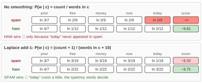
“today” appears in ham emails but never in a spam email. Without smoothing P(today | spam) = 0/9 = 0, and one zero in a product makes the whole product 0. The email “free money now today” then scores 0 for spam, whatever “free money now” says, and lands in the inbox (Demo 3).

Laplace (add-1) smoothing pretends every word was seen once more in every class: P(w | c) = (count + 1) / (words in c + |V|). Now P(today | spam) = 1/19: small, but not zero, and the other words can still win. Each class's likelihoods still add up to 1, because the +1 on all 10 words is matched by +10 in the denominator.

“free money now today”	spam	ham	verdict
no smoothing	−∞ (“today” never in spam)	−9.81	ham ✗
add-1	−9.33	−9.75	spam ✓

Add-1 is the simplest choice. Real filters often add a smaller α (Lidstone smoothing, e.g. 0.1), so rare words are not pulled as hard towards uniform.

Underflow: why add logs instead of multiplying

Every likelihood is a small number, around 0.05 to 0.2. A real email has hundreds of words, and the product of hundreds of such numbers is something like 10⁻⁴⁰⁰. A 64-bit double cannot hold anything below about 5 × 10⁻³²⁴, so the product becomes exactly 0 (see Floating Point for where that limit comes from). In Demo 4 the 600-word email underflows to 0 for both classes, and 0 = 0 leaves the filter unable to decide.

The fix is to take logarithms: ln(a × b) = ln a + ln b, and ln is increasing, so the class with the larger product also has the larger sum of logs.

score(c) = ln P(c) + Σ count(w) × ln P(w | c)

The same 600-word email scores −1108.4 for spam and −1543.3 for ham: ordinary numbers, and the right answer. Every real implementation works in log space.

Borderline emails and the posterior

The difference between the two scores is a confidence. From the log scores you get the posterior back with P(spam | email) = 1 / (1 + eham − spam). For “free lunch now” the scores are −7.48 and −7.35, so P(spam | email) ≈ 0.47: a coin flip (Demo 5). Filters therefore use a threshold well above 0.5 (often 0.9 or more) before moving a mail to the spam folder, because losing a real email is worse than letting one spam through.

Naive Bayes is known to be overconfident: because correlated words are counted as independent evidence, its posteriors pile up near 0 and 1. The ranking is useful; the exact number is not.

See also Bayesian Networks for Bayes' rule with dependencies between variables, k-Nearest Neighbors and Decision Trees for other simple classifiers, Linear and Logistic Regression for the discriminative cousin of Naive Bayes, and BPE Tokenizer for how modern models split text into tokens instead of whole words.

See Bayes' Theorem for the rule itself, counted on 1000 people taking a medical test.

See also Precision vs Recall, which thresholds a spam filter's scores and shows what each threshold costs in lost email and missed spam.

What the page leaves out

Tokenizing real emails (case, punctuation, stemming, stop words, headers and URLs); the Bernoulli model, which records only whether a word occurs; smoothing with α other than 1; words seen only at test time growing the vocabulary; feature selection and TF-IDF weighting; more than two classes (the same formula, one row per class); and continuous features, where Gaussian Naive Bayes uses a normal distribution per feature instead of counts.

References

Jurafsky & Martin, Speech and Language Processing, ch. 4: Naive Bayes and Sentiment Classification

Manning, Raghavan & Schütze, Introduction to Information Retrieval: Naive Bayes text classification

scikit-learn: Naive Bayes (MultinomialNB, alpha)