The idea: count the people who test positive
A disease affects 1% of people. A test finds 90% of the sick, and wrongly flags 9% of the healthy. You test positive. How likely is it that you are sick? Most people guess about 90%. The answer is about 9%.
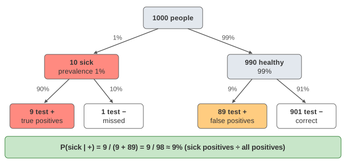
The page shows why by counting. Each square in the 40 × 25 grid is one person. 10 are sick. 9 of them test positive. Of the 990 healthy people, 89 also test positive. A positive result puts you in a group of 98 people, and only 9 of those 98 are sick (Demo 1).
Bayes' theorem is the same count
Bayes' theorem turns one conditional probability around:
P(A | B) = P(B | A) · P(A) / P(B)

P(sick | +) = P(+ | sick) · P(sick) / P(+)
            =  (9/10)     · (10/1000) / (98/1000)
            =  9/98  ≈ 0.092
Each factor has a name, and each is a fraction of the grid:
| term | name | count on the grid | value |
|---|---|---|---|
P(sick) | prior (prevalence) | 10 sick / 1000 people | 0.010 |
P(+ | sick) | likelihood (sensitivity) | 9 positive / 10 sick | 0.90 |
P(+) | evidence | 98 positive / 1000 people | 0.098 |
P(sick | +) | posterior | 9 sick / 98 positive | 0.092 |
Multiply the first two and the 10s cancel: 9/10 · 10/1000 = 9/1000, the share of all people who are sick and positive. Dividing by 98/1000 keeps only the positives. So the theorem says: sick positives ÷ all positives.
The evidence: two ways to test positive
P(+) is rarely given directly. You build it from both groups, with the law of total probability:
P(+) = P(+ | sick) · P(sick) + P(+ | healthy) · P(healthy)
     = 0.90 · 0.01 + 0.09 · 0.99  =  0.0981   (98 of 1000 people)
The second term is the false positives. When the disease is rare, there are many more healthy people to make mistakes on, so the false positives dominate even with a good test. The formula panel on the page writes this sum out with the grid counts.
A second test: the posterior becomes the prior
Now only the 98 positives take a second, independent test (Demo 2). Among them 9 are sick, so the prior is no longer 1% but 9/98 ≈ 9%. 8 of the 9 sick test positive again, but only 8 of the 89 healthy are unlucky twice. That leaves 16 people, half of them sick: P(sick | + +) = 8/16 = 50%.
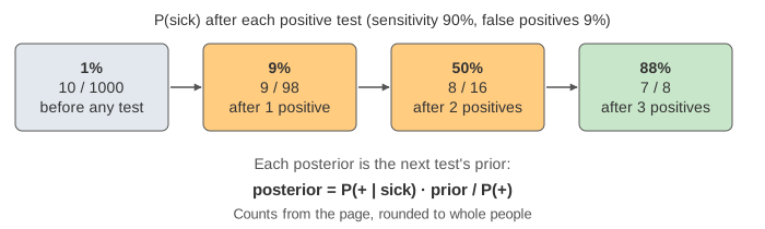
This is Bayesian updating: the same formula, applied again with yesterday's posterior as today's prior. In odds form each positive result multiplies the odds by the likelihood ratio P(+ | sick) / P(+ | healthy) = 0.90 / 0.09 = 10: odds 1:99 become 10:99, then 100:99. The tests must be independent given the true state; repeating the same test on the same faulty sample does not count twice.
Base rate versus test quality
Change the dropdowns and test again. The posterior depends as much on how common the disease is as on how good the test is:
| prevalence | P(+ | sick) | P(+ | healthy) | positives | P(sick | +) |
|---|---|---|---|---|
| 0.1% | 90% | 9% | 1 + 90 | 1% |
| 1% | 90% | 9% | 9 + 89 | 9% |
| 10% | 90% | 9% | 90 + 81 | 53% (Demo 3) |
| 50% | 90% | 9% | 450 + 45 | 91% |
| 1% | 99% | 1% | 10 + 10 | 50% (Demo 4) |
A much better test at 1% prevalence (Demo 4) only reaches 50%: the 1% false-positive rate, on 990 healthy people, still makes as many false alarms as there are sick people. This is why screening a whole population for a rare disease needs a second, confirming test, and why a test given to people with symptoms (a higher prior) is far more convincing.
The base-rate fallacy
P(+ | sick) and P(sick | +) look alike but count different groups. The first looks inside the sick: 9 of 10 test positive. The second looks inside the positives: 9 of 98 are sick (Demo 5). Answering 90% to "how likely am I sick?" swaps the two and ignores the base rate, the 1% prevalence. The same mistake appears in courtrooms (the prosecutor's fallacy: "the chance of a random match is 1 in a million" is not "the chance the defendant is innocent") and in alarms and spam filters with rare events.
Drawing the people, as the page does, is the standard cure: with natural frequencies ("9 of 98") most people get the answer right, while with percentages most get it wrong.
See also Naive Bayes, which applies the same theorem to classify emails from word counts, Bayesian Networks, which chain many such updates through a graph of causes, A/B Testing for false positives in experiments, and Monte Carlo π for estimating probabilities by counting random samples.
See also Precision vs Recall: precision is P(sick | flagged), and the rare-disease demo shows why accuracy misleads when positives are rare.
See also hypothesis testing: a false positive is a type I error, and a p-value is P(data | H₀), not P(H₀ | data).
See also the Monty Hall problem, where the same prior × likelihood ÷ evidence step (likelihoods 1/2, 1, 0 for "Monty opens door 3") turns 1/3 into 2/3.
What the page leaves out
Rounding: the grid counts whole people, so its fractions differ slightly from the exact ones (the exact second-test posterior is 50.2%, the grid shows 8/16). Continuous priors and likelihoods (Bayes' theorem with densities, as in Bayesian statistics); conjugate priors such as Beta–Binomial; the odds form and likelihood ratios beyond one sentence; tests that are not independent; specificity as a separate term (here it is 1 − the false-positive rate, 91%); confidence about the prevalence itself; and the debate between Bayesian and frequentist statistics.