The idea: undo A with row operations
The inverse A⁻¹ of a square matrix A is the matrix that undoes it: A⁻¹·A = I, so A⁻¹ sends every point A moved back where it came from. One way to find it is row reduction: write A and the identity I side by side as the augmented matrix [A | I], and do row operations on both halves until the left half is I. The right half is then A⁻¹.
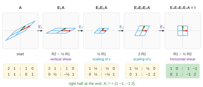
On the canvas the blue grid is the plane after the left half of the augmented matrix: at the start that is A, so î sits at A's first column and ĵ at its second. Each row operation moves that grid, the grey grid shows where it was, and when the left half reaches I the blue grid is the plain square grid again (Demo: undo A with row operations).
Row operations are matrices
Every row operation is the same as multiplying on the left by an elementary matrix E: the identity with that one operation done to it. Doing the operation to [L | R] gives [E·L | E·R]. And because E multiplies on the left, it acts on the grid of L as a map of the plane in its own right. There are three kinds:
| Row operation | E | What E does to the plane |
|---|---|---|
| R2 ← R2 + c·R1 | [1 0; c 1] | vertical shear: (x, y) → (x, y + c·x) |
| R1 ← R1 + c·R2 | [1 c; 0 1] | horizontal shear: (x, y) → (x + c·y, y) |
| R1 ← s·R1 (s ≠ 0) | [s 0; 0 1] | scaling of x by s (a flip too if s < 0) |
| R2 ← s·R2 (s ≠ 0) | [1 0; 0 s] | scaling of y by s |
| R1 ↔ R2 | [0 1; 1 0] | reflection in the line y = x: (x, y) → (y, x) |
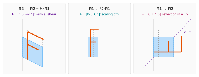
With A = [1 −1; 1 1] (a turn by 45° and a stretch by √2) the steps are R2 ← R2 − R1 (a vertical shear), R2 ← ½·R2 (squash y by ½) and R1 ← R1 + R2 (a horizontal shear). No rotation is needed to undo a rotation: shears and scalings are enough (Demo: each row operation is a shear or a scaling). The in-between frames on the canvas are I + t(E − I), so the grid really goes through the partial shear or scaling.
A row swap is a reflection
For A = [0 2; 1 1] the pivot spot (row 1, column 1) holds 0, and nothing can be divided by 0. Swapping the rows fixes that. Its matrix [0 1; 1 0] swaps the coordinates of every point, the mirror image in the line y = x. On the canvas each point goes straight across the purple mirror line at a right angle, so halfway the whole grid lies on that line: a reflection reverses orientation (det = −1) and cannot be done by a smooth motion inside the plane (Demo: a row swap is a reflection).
The right half records A⁻¹
Say k row operations E₁, E₂, …, Eₖ bring the left half to I. Then
The right half started as I and got exactly the same operations, so it holds Eₖ⋯E₂E₁·I = A⁻¹. Nobody has to multiply the E's out: the augmented matrix does it as it goes. For A = [2 1; 1 1] the four steps give A⁻¹ = [1 −1; −1 2], and indeed A·A⁻¹ = [2·1 + 1·(−1) 2·(−1) + 1·2; 1·1 + 1·(−1) 1·(−1) + 1·2] = I. The order is the reverse of the order the maps happen in, as in any product of maps (see Matrix Multiplication and Composing Transforms). Read the other way, A = E₁⁻¹E₂⁻¹⋯Eₖ⁻¹: every invertible matrix is a product of shears, scalings and swaps.
The 2×2 formula as a check
For a 2×2 matrix there is a shortcut: swap the diagonal entries, change the signs of the other two, and divide by the determinant:
For [2 1; 1 1]: det = 2·1 − 1·1 = 1, so A⁻¹ = [1 −1; −1 2], the same as the right half (Demo: check with the 2×2 formula). For [0 2; 1 1]: det = −2 and (1/−2)·[1 −2; −1 0] = [−½ 1; ½ 0]. The formula is handy for 2×2; row reduction is what works for any size (see Gaussian Elimination).
When there is no inverse: det = 0
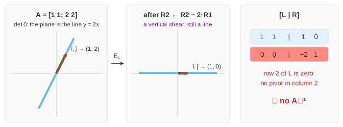
A = [1 1; 2 2] sends î and ĵ both to (1, 2): the whole plane is squashed onto the line y = 2x, and det A = 1·2 − 1·2 = 0. Row reduction finds it at once: R2 ← R2 − 2·R1 leaves the row (0, 0 | −2, 1). The left half has a zero row, there is no pivot in column 2, and no row operation can make one. On the canvas the grid stays flat: a shear moves the line onto the x-axis, but no shear, scaling or swap can open a line out into a plane again. Two different points went to the same place, so no matrix can send them back (Demo: singular: a zero row, no inverse). The formula agrees: it would divide by 0.
| A | det A | row operations | A⁻¹ |
|---|---|---|---|
| [2 1; 1 1] | 1 | R2 − ½R1, ½R1, 2R2, R1 − ½R2 | [1 −1; −1 2] ✓ |
| [1 −1; 1 1] | 2 | R2 − R1, ½R2, R1 + R2 | [½ ½; −½ ½] ✓ |
| [0 2; 1 1] | −2 | R1 ↔ R2, ½R2, R1 − R2 | [−½ 1; ½ 0] ✓ |
| [1 1; 2 2] | 0 | R2 − 2R1, then a zero row | none ✗ |
See also the overview Linear Transformations, the single maps Shear Matrix, Scaling Matrix, Reflection Matrix and Rotation Matrix, products of maps in Composing Transforms, why det 0 means a lost direction in Determinant and Column Space and Null Space, and solving systems with the same row operations in Gaussian Elimination.
What the page leaves out
Only 2×2 matrices and one fixed order of row operations are shown; other orders give other E's but the same A⁻¹. Larger matrices work the same way with n×n elementary matrices. Partial pivoting (swapping in the largest pivot to keep rounding errors small), the LU factorization (keeping the E's instead of applying them), the cost (about n³ operations), and why one should usually solve A·x = b directly rather than form A⁻¹ are left out, as are left and right inverses of non-square matrices and the pseudo-inverse.