Gram–Schmidt: Orthonormal Vectors and A = QR

The idea: subtract the shadows, then normalize

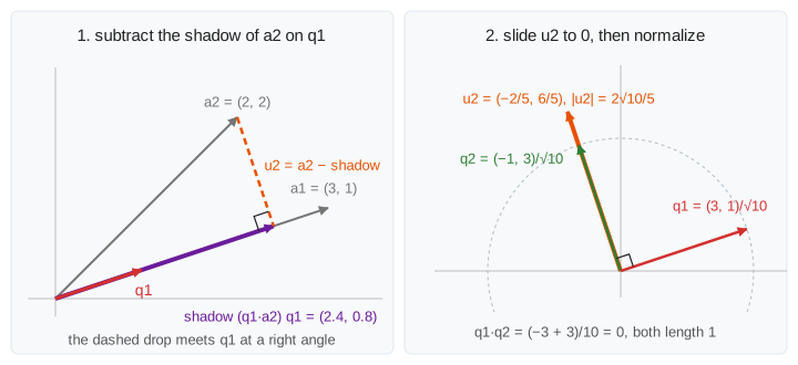
Vectors a₁, a₂, a₃ can span a space and still be awkward to work with: they lean on each other and have all sorts of lengths. The Gram–Schmidt process replaces them with vectors q₁, q₂, q₃ that span the same space but are orthonormal: each has length 1 and each is perpendicular to the others. The recipe is one sentence: take the next vector, subtract its shadows on the q's you already have, and normalize what is left.

The steps, one vector at a time

1. q₁ = a₁ / |a₁|. Nothing to subtract yet; just make it length 1.
2. u₂ = a₂ − (q₁·a₂) q₁, then q₂ = u₂ / |u₂|.
3. u₃ = a₃ − (q₁·a₃) q₁ − (q₂·a₃) q₂, then q₃ = u₃ / |u₃|.

The shadow of a on a unit vector q is (q·a) q: the foot of the perpendicular dropped from the tip of a onto q's line, exactly as on the Projection Matrix page. What is left, the remainder u, is the dashed drop itself, so it meets q at a right angle. You can check it in one line: q₁·u₂ = q₁·a₂ − (q₁·a₂)(q₁·q₁) = 0, because q₁·q₁ = 1. For a₃ the two shadows add up to its shadow on the plane of q₁ and q₂, and the drop is perpendicular to that whole plane. (Demo 1: Two vectors in 2D, Demo 2: Three vectors in 3D)

The start example, worked out exactly:

vector	remainder u	|u|	q
a1 = (0, 1, 1)	(0, 1, 1)	√2	(0, 1, 1)/√2
a2 = (1, 0, 1)	a2 − ½(0, 1, 1) = (1, −½, ½)	√6/2	(2, −1, 1)/√6
a3 = (1, 1, 0)	a3 − (0, ½, ½) − (1/3, −1/6, 1/6) = (2/3, 2/3, −2/3)	2√3/3	(1, 1, −1)/√3

Q and R: A = QR

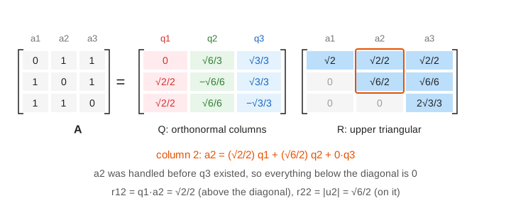
Read the steps backwards: every a_j is rebuilt from the q's. a₁ = r₁₁ q₁, a₂ = r₁₂ q₁ + r₂₂ q₂, a₃ = r₁₃ q₁ + r₂₃ q₂ + r₃₃ q₃, where the numbers are the ones the process used:

• r_ij = q_i·a_j above the diagonal (how far a_j reaches along q_i),
• r_jj = |u_j| on the diagonal (the length of what was left).

Put the a's as the columns of A, the q's as the columns of Q and the numbers in R: that is A = QR. R is upper triangular because a_j only uses q₁ … q_j; the later q's were not made yet when a_j was handled. For the start example R = [√2, √2/2, √2/2; 0, √6/2, √6/6; 0, 0, 2√3/3]. The page fills Q and R entry by entry, then rebuilds each column of A to check. (Demo 3: Build Q and R, check A = QR)

QᵀQ = I

Entry (i, j) of QᵀQ is q_i·q_j: 1 when i = j (unit length) and 0 otherwise (perpendicular). So QᵀQ = I, and when Q is square Q⁻¹ = Qᵀ: undoing Q costs only a transpose. Multiplying by Q keeps lengths and angles, which is why numerical methods like it. (Demo 6: Check: QᵀQ = I)

A dependent vector leaves nothing

Take a₃ = a₁ + a₂ = (1, 1, 2). It lies in the plane of q₁ and q₂, so its shadow on that plane is the whole vector: a₃ = (3√2/2) q₁ + (√6/2) q₂, and the remainder is u₃ = 0. There is nothing to normalize, so there is no q₃, r₃₃ = 0, and the rank is 2, not 3. A zero remainder is how Gram–Schmidt finds out that a vector depends on the ones before it. (Demo 4: A dependent vector leaves nothing)

Nearly parallel vectors: cancellation

a₁ = (4, 1) and a₂ = (5, 1) are about 2.7° apart. Almost all of a₂ is its shadow: (q₁·a₂) q₁ = (21/17)(4, 1), and the remainder u₂ = (1/17, −4/17) has length √17/17 ≈ 0.24, about 4.8% of |a₂| ≈ 5.1. Exactly, that is fine. In floating point it is not: subtracting two nearly equal numbers keeps their rounding errors but loses the leading digits, so the computed q₂ can be visibly not perpendicular to q₁. Libraries use modified Gram–Schmidt (subtract one shadow at a time from the updated vector) or Householder reflections instead. (Demo 5: Nearly parallel: a tiny remainder)

Where QR is used

• Least squares: to fit Ax ≈ b, write A = QR. The normal equations AᵀAx = Aᵀb become Rx = Qᵀb, solved from the bottom up because R is triangular, without forming AᵀA (see Least Squares).
• The QR algorithm for eigenvalues: factor A = QR, multiply back the other way RQ, repeat. The matrices keep the same eigenvalues and approach a triangular one with the eigenvalues on its diagonal (see Eigenvectors).
• An orthonormal basis for a column space, for projections (P = QQᵀ) and for changing coordinates.

See also Linear Transformations, Vectors and the Dot Product, Projection Matrix and its 3D version Projection onto a Plane, Column Space and Null Space, Gaussian Elimination (A = LU, the other triangular factorization), Matrix Multiplication, Inverse Matrix, Rotation Matrix and 3D Rotation Matrix (orthogonal matrices), 3D Reflection Matrix, SVD and PCA and Diagonalization.

What the page leaves out

Modified Gram–Schmidt, re-orthogonalization and the Householder and Givens ways to compute QR, which are what numerical libraries use. Floating-point error itself (the page keeps every number exact). Pivoting to handle dependent columns, the full versus reduced QR (a square Q with extra columns when A is tall), more than three vectors, complex vectors, other inner products (Gram–Schmidt on functions gives the Legendre polynomials) and the shifted QR algorithm.

References

Gilbert Strang, MIT 18.06 Lecture 17: Orthogonal matrices and Gram–Schmidt

Gram–Schmidt process (Wikipedia)

QR decomposition (Wikipedia)