The idea: two rules, two pictures
Most integrals are not in a table. Two techniques turn them into ones that are. Integration by parts is the product rule read backwards: ∫u dv = [uv] − ∫v du. Substitution (u-substitution) is the chain rule read backwards: ∫f(g(x)) g′(x) dx = ∫f(u) du with u = g(x). Both rules have a picture. By parts says that one rectangle is cut by a curve into two areas. Substitution says that stretching the axis under an area, and squashing its height by the same factor, leaves the area alone.
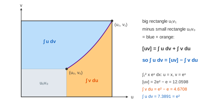
Integration by parts: one rectangle, two areas
Pick u and v as functions of a parameter t (for ∫x eˣ dx: u = x, v = eˣ) and plot the point (u, v) as t runs over the interval. Take the rectangle from the origin to the end point (u₁, v₁) and remove the one to the start point (u₀, v₀). What is left, [uv] = u₁v₁ − u₀v₀, is split by the curve into two pieces:
- between the curve and the v-axis: horizontal strips of length u and thickness dv, total ∫u dv (blue);
- between the curve and the u-axis: vertical strips of height v and width du, total ∫v du (orange).
The two pieces fill the L-shape with no gap and no overlap, so ∫u dv + ∫v du = [uv]. The same rule comes from the product rule: d(uv) = u dv + v du, integrated from start to end. The picture needs u and v to increase together; in general the areas are signed, and the formula holds anyway.
Worked examples
| integral | u, dv | [uv] | ∫v du | ∫u dv |
|---|---|---|---|---|
| ∫₀¹ x eˣ dx | u = x, dv = eˣ dx | 1·e − 0·1 = 2.7183 | e − 1 = 1.7183 | 1 |
| ∫₁² x eˣ dx | u = x, dv = eˣ dx | 2e² − e = 12.0598 | e² − e = 4.6708 | e² = 7.3891 |
| ∫₁ᵉ ln x dx | u = ln x, dv = dx | 1·e − 0·1 = 2.7183 | ∫₁ᵉ x·(1/x) dx = e − 1 | 1 |
For ∫₀¹ x eˣ dx the start point is (0, 1), so the small rectangle is flat (u₀ = 0) and the whole rectangle 1 × e is shared: e = 1 + (e − 1) (Demo: by parts, ∫₀¹ x eˣ dx = 1). On [1, 2] the start point is (1, e) and the grey rectangle u₀v₀ = e is cut away first, leaving an L-shape (Demo: by parts with an L-shape). For ∫ln x dx the trick is to take dv = dx, so v = x and v du = x·(1/x) dx = dx is trivial. Its curve (ln t, t) is the same curve as (t, eᵗ), because ln and exp are inverse functions, so the picture is the same as the first example (Demo: by parts, ∫₁ᵉ ln x dx = 1).
A rule of thumb for choosing u is LIATE: Logarithms, Inverse trig, Algebraic, Trig, Exponential. Choose u from early in the list, so that du is simpler than u, and dv from late in the list, so that v is easy to find.
Substitution: stretch the axis, keep the area
In ∫f(g(x)) g′(x) dx, set u = g(x). Cut the x-interval into strips of width dx. The map u = g(x) sends each strip to a u-strip of width du ≈ g′(x)·dx. On the u-axis give the strip the height f(u) = f(g(x)). Its area f(g(x))·g′(x)·dx is the same as before: the factor g′(x) moved from the height into the width. Adding up all the strips:
∫ab f(g(x)) g′(x) dx = ∫g(a)g(b) f(u) du.
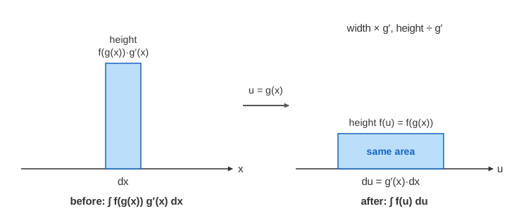
Where g′ > 1 the axis is stretched and the strips get wider and lower; where g′ < 1 it is squeezed and they get narrower and taller. The canvas draws the x-plot and the u-plot at the same scale, so the stretch is the real one. Each box is drawn at its strip's average height, so it has the strip's exact area, and the info panel shows that the boxes on the two plots add up to the same total.
| integral | u = g(x) | new limits | result |
|---|---|---|---|
| ∫0√π 2x sin(x²) dx | u = x², du = 2x dx | 0 → π | ∫0π sin u du = −cos π + cos 0 = 2 |
| ∫0π/2 cos x·esin x dx | u = sin x, du = cos x dx | 0 → 1 | ∫₀¹ eᵘ du = e − 1 = 1.7183 |
For u = x² the strips near √π are stretched about 3.25 times: the last of 6 strips has dx = 0.2954 and du = 0.9599 (Demo: substitution stretches). For u = sin x, g′ = cos x falls to 0 at π/2, so the last strip is squeezed to almost nothing and becomes a tall thin box (Demo: substitution squeezes). With 12 strips the boxes are thinner but the totals still agree (Demo: 12 thinner strips).
Two habits make substitution safe. Change the limits with u (x = √π becomes u = π), so you never have to go back to x. And check that the whole integrand is used: the g′(x) dx must be there, possibly up to a constant factor, or the substitution does not apply.
See also
The Fundamental Theorem of Calculus explains why finding an antiderivative gives the area at all. The chain rule is the derivative rule that substitution reverses. Riemann sums are the strips used here, and accumulation reads an integral as a running total. Improper integrals often need these techniques first, for example ∫0∞ x e−x dx by parts. The derivative rules include the product rule behind integration by parts.
When no antiderivative can be found, estimate the integral instead: Numerical Integration: Riemann vs Trapezoid vs Simpson.
What the page leaves out
Indefinite integrals and the constant +C, repeated integration by parts (∫x² eˣ dx) and the tabular method, by parts that comes back to the start (∫eˣ sin x dx), curves where u or v decreases (signed areas), trigonometric and inverse substitutions (x = sin θ), partial fractions, and substitutions where g is not monotone.