Numerical Integration: Riemann vs Trapezoid vs Simpson

The idea: same strips, three shapes

Most integrals have no formula you can write down, so computers estimate them. All three rules on this page do it the same way: cut [a, b] into n strips of width h = (b − a)/n, evaluate f at the strip ends (the nodes), fit a simple shape whose area is easy, and add the areas. They differ only in the shape. The left Riemann sum uses a flat rectangle, the trapezoid rule a straight line between the two ends, and Simpson's rule a parabola through three nodes for every pair of strips.

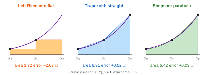
The canvas runs the three rules in lockstep on the same curve: one Step adds the next strip (or parabola piece) in every lane, with a running sum S. When a run ends, each lane shows its error, ★ marks the closest, and a point per lane goes onto the log-log chart below. Press Double n to add the next point. (Demo: sin x on [0, π], n = 4)

Left Riemann sum: rectangles

Each strip gets the height of f at its left end: S = h·(f(x₀) + f(x₁) + … + f(x_n−1)). That is n evaluations of f. A flat top misses the slope of the curve, so each strip is off by about ½·f′·h², and n strips add up to an error of about ½·(f(b) − f(a))·h. The error is proportional to h: doubling n only halves it. See Riemann Sums for the right and midpoint versions.

Trapezoid rule: straight lines

Each strip gets the average of its two end heights: S = h·(½f(x₀) + f(x₁) + … + f(x_n−1) + ½f(x_n)). That is n + 1 evaluations, one more than the Riemann sum. A straight top follows the slope and misses only the bend, so the error is about −(b − a)·h²·f″/12: proportional to h². Doubling n divides it by 4. It is also the average of the left and right Riemann sums.

Simpson's rule: parabolas

Simpson takes the strips in pairs. Through the three nodes of a pair it draws the one parabola that passes through all three, and adds its area, (h/3)·(f₀ + 4f₁ + f₂). Over all pairs the weights are 1, 4, 2, 4, 2, …, 4, 1, times h/3. It needs n even and the same n + 1 evaluations as the trapezoid. Its error is about −(b − a)·h⁴·f⁗/180: proportional to h⁴, so doubling n divides it by 16. Because the error has f⁗ in it, Simpson is exact for every cubic, not only for parabolas. (Demo: Simpson is exact on x³)

Simpson is also (4·T_2n − T_n)/3, two trapezoid sums combined so that their h² errors cancel. Repeating that trick is Romberg integration.

Error order on a log-log chart

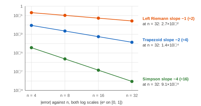
If the error is C·h^p, then log|error| = log C − p·log n + constant: a straight line with slope −p when both axes are logarithmic. The chart under the lanes is drawn that way, and the scoreboard next to it prints the measured ÷ per doubling and the order p = log₂(÷). On eˣ the three lines fall with slopes −1, −2 and −4. (Demo: error order on eˣ, n = 4 → 32)

eˣ on [0, 1]	Left Riemann	Trapezoid	Simpson
n = 4	−0.2058	+0.0089	+3.70×10⁻⁵
n = 8	−0.1052	+0.0022	+2.33×10⁻⁶
n = 16	−0.0531	+0.00056	+1.46×10⁻⁷
n = 32	−0.0267	+0.00014	+9.10×10⁻⁹
÷ per doubling	≈ 2 (order 1)	≈ 4 (order 2)	≈ 16 (order 4)

When the order breaks

The error formulas assume f has enough smooth derivatives. Two cases on the page break that assumption, in opposite directions.

• √x on [0, 1] has an infinite slope at 0. The first strip is badly fitted by every shape, and that one strip dominates. Trapezoid and Simpson both fall to about order 1.5 (÷ 2.8 per doubling). Simpson still wins, but only by a factor of about 2.5, not thousands. (Demo: non-smooth √x, n = 4 → 32)
• 1/(2 + cos x) on [0, 2π] is smooth and periodic. Over a whole period the trapezoid's errors cancel almost perfectly, and its error shrinks faster than any power of h: 5×10⁻⁹ at n = 16, while Simpson is still at 6×10⁻⁵. Simpson's uneven 1, 4, 2, 4 weights break the cancellation. The left Riemann sum equals the trapezoid here, because f(0) = f(2π). (Demo: periodic, the trapezoid beats Simpson)

The same thing happens in a small way on sin x over [0, π]: sin 0 = sin π = 0, so the left Riemann sum and the trapezoid give the same 1.8961 at n = 4, both O(h²) here.

When to pick which

	Left Riemann	Trapezoid	Simpson
Shape on a strip	flat	straight line	parabola over 2 strips
f evaluations	n	n + 1	n + 1 (n even)
Error, smooth f	∝ h	∝ h²	∝ h⁴
Exact for	constants	straight lines	cubics
Best at	defining the integral; data that comes as running totals	periodic functions over a full period; measured data at uneven spacing	smooth functions you can evaluate anywhere

The exact value without any sum, and why adding up f·h gives the area at all, is on the Fundamental Theorem of Calculus. When an antiderivative does exist, Integration Techniques finds it by parts or by substitution. Random points instead of strips: Monte Carlo estimation of π, whose error shrinks only like 1/√n but does not care about the dimension.

What the page leaves out

The midpoint rule (order 2, half the trapezoid's error, see Riemann Sums), Gaussian quadrature, which places the nodes at unequal points and gets order 2n from n of them, adaptive methods that add strips only where the curve bends most, Romberg extrapolation beyond one step, integrals over infinite ranges, multiple integrals, and floating-point rounding, which stops every rule from improving once its error nears 10⁻¹⁶.

References

OpenStax Calculus Volume 2, 3.6 Numerical Integration (error bounds for the midpoint, trapezoid and Simpson rules)

Wikipedia: Simpson's rule

Trefethen and Weideman, The exponentially convergent trapezoidal rule (SIAM Review, 2014)