The idea: five numbers and a fence
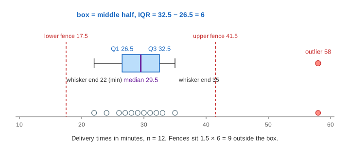
A box plot draws a data set with five numbers: the minimum, the lower quartile Q1, the median, the upper quartile Q3 and the maximum. The box runs from Q1 to Q3, so it holds the middle half of the values. Its width is the interquartile range, IQR = Q3 − Q1. Two fences sit 1.5 × IQR outside the box. A value beyond a fence is called an outlier and is drawn as a single point; the whiskers stop at the last values inside the fences. The page builds all of this one Step at a time, then tries a second rule, the z-score rule, on the same data.
Quartiles by the median of halves
Quartiles are about order, so the first Step sorts the values. The median Q2 is the middle value (odd n) or the average of the middle two (even n). It splits the list into a lower and an upper half. Q1 is the median of the lower half and Q3 the median of the upper half. When n is odd, this page leaves the median out of both halves. For the 11 exam scores the median 73 is the 6th value, each half has 5 values, and Q1 = 68, Q3 = 79 (Demo: exam scores). For the 12 delivery times each half has 6 values, so Q1 and Q3 are averages: (26 + 27) ÷ 2 = 26.5 and (32 + 33) ÷ 2 = 32.5.
About a quarter of the values lie below Q1 and about a quarter above Q3. The IQR is not moved by how far out the extreme values are: change 58 to 580 and the box stays the same. That is why the fences are built from it. The median and why it resists outliers are on Mean vs Median vs Mode.
Quartile methods differ
There is no single agreed formula for quartiles; Hyndman and Fan list nine. The second dropdown switches this page to linear interpolation: Q sits at position (n − 1) × p in the sorted list counted from 0, between two values when the position is not whole. This is the default of NumPy's percentile, Excel's QUARTILE.INC and R's quantile (type 7). On large data sets the methods barely differ. On small ones they can change the verdict for a value near a fence. For the ten values 10, 12, 13, 14, 15, 16, 17, 19, 20, 28:
| Method | Q1 | Q3 | IQR | Upper fence | Is 28 an outlier? |
|---|---|---|---|---|---|
| Median of halves (this page; TI calculators) | 13 | 19 | 6 | 28 | no, it is on the fence ✓ |
| Tukey's hinges (median kept in both halves when n is odd) | 13 | 19 | 6 | 28 | no (n is even, so same as above) |
| Linear, position (n − 1)p: NumPy, Excel QUARTILE.INC, R type 7 | 13.25 | 18.5 | 5.25 | 26.375 | yes ✗ |
| Position (n + 1)p: Excel QUARTILE.EXC, R type 6, Minitab | 12.75 | 19.25 | 6.5 | 29 | no |
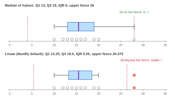
So when you report outliers, say which method you used (Demo: a value exactly on the fence and Demo: same data, linear quartiles).
Fences, whiskers and outliers
The lower fence is Q1 − 1.5 × IQR and the upper fence Q3 + 1.5 × IQR. For the deliveries that is 26.5 − 9 = 17.5 and 32.5 + 9 = 41.5, so the 58-minute delivery is an outlier (Demo: one late delivery). Three details are easy to get wrong:
- The whisker ends at the last data value inside the fence (35 here), not at the fence itself. Most box plots do not draw the fences at all.
- Only values beyond a fence are outliers. A value exactly on it stays in, and the whisker reaches it.
- With no outliers, the whiskers reach the minimum and the maximum, and the box plot shows exactly the five-number summary.
The factor 1.5 is Tukey's choice. For normal data it puts the fences about 2.7 standard deviations from the centre, so only about 0.7% of normal values land outside. Values beyond 3 × IQR are sometimes called far out or extreme outliers.
The z-score rule and why it can fail
The other common rule standardises each value, z = (x − mean) / s, and calls it an outlier when |z| > 3; z-scores are explained on Normal Distribution and s on Variance and Standard Deviation. The page uses the sample s, dividing by n − 1. The rule has three weak points, and the demos show each:
- Masking. The outlier is part of the mean and s it is measured against. The late delivery pulls the mean from 28.8 (without it) to 31.25 and more than doubles s, to 9.22, so its own z is only 2.90 and it is not flagged.
- Small samples. No value can have |z| larger than (n − 1) / √n. For n = 10 that is 2.85, so with ten values the rule |z| > 3 can never flag anything, however wild the value.
- Skew. The rule assumes a roughly normal, symmetric shape. The response times have a long right tail: s is 150.9 ms, mean − 3s is −275.7 ms, an impossible time, and 400 ms has z = 1.48. Only 650 (z = 3.13) is flagged, while the IQR rule flags both 400 and 650 (Demo: skewed response times).
Which rule when
| IQR rule (1.5 × IQR fences) | z-score rule (|z| > 3) | |
|---|---|---|
| Built from | quartiles: order only | mean and s: every value's size |
| Moved by the outliers themselves | hardly ✓ | yes, they hide themselves ✗ |
| Small n | works, but depends on the quartile method | cannot flag anything when n ≤ 10 ✗ |
| Skewed data | flags much of the long tail, which may be real | band can reach impossible values ✗ |
| Use it for | a first look at any data set, with a box plot | large, roughly normal data |
An outlier flag is a reason to look, not to delete. The 58-minute delivery may be a typo, a lost parcel or a real rush-hour trip; slow response times in a long tail are often the most important ones. For skewed data, a box plot of the logarithm of the values is often a fairer picture.
What the page leaves out
Side-by-side box plots for comparing groups, notched box plots (a confidence interval for the median), variable-width and violin plots, adjusted box plots for skewed data (the medcouple), the median absolute deviation (MAD) and the modified z-score, formal outlier tests (Grubbs, Dixon), percentiles other than the quartiles, and quartiles of grouped data or of a continuous distribution.