The idea: is this die fair?
You roll a die 60 times and get 20 sixes. A fair die should give about 10. Is it loaded, or was that luck? The data are counts in categories (how many 1s, 2s, … 6s), not one number like a coin's heads. The chi-square test turns the six counts into one number and asks how surprising it would be from a fair die.
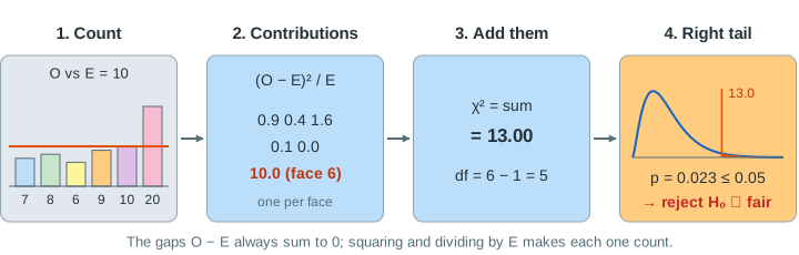
On the canvas, the bars show the observed counts against the orange line E = 10, the die grid shows every roll, the table does the arithmetic, and the bottom chart is how χ² falls when the die is fair.
Observed and expected counts
The null hypothesis H₀ gives a probability to every category: here 1/6 per face. The expected count is E = n × probability = 60 × 1/6 = 10. The observed counts O are what the rolls produced. Even a fair die never gives exactly 10 of each; the question is whether the gaps O − E are bigger than chance usually makes them.
The statistic χ² = Σ (O − E)² / E
The gaps O − E always add up to 0 (too many sixes means too few of something else), so their sum is useless. The test squares each gap, so too many and too few both count, and divides by E, so a gap of 5 on an expected 10 weighs more than a gap of 5 on an expected 1000. Then it adds the six contributions:
| face | O | E | O − E | (O − E)²/E |
|---|---|---|---|---|
| 1 | 7 | 10 | −3 | 0.90 |
| 2 | 8 | 10 | −2 | 0.40 |
| 3 | 6 | 10 | −4 | 1.60 |
| 4 | 9 | 10 | −1 | 0.10 |
| 5 | 10 | 10 | 0 | 0.00 |
| 6 | 20 | 10 | +10 | 10.00 |
| χ² = sum | 13.00 | |||
One face with a big gap dominates (Demo: 20 sixes → reject H₀). But many small gaps add up too: counts 5, 15, 6, 14, 5, 15 have no gap above 5, yet χ² = 13.20 (Demo: many small gaps add up). A die that looks fair, 8, 12, 9, 11, 10, 10, gives only χ² = 1.00 (Demo: a fair-looking die → keep H₀).
Degrees of freedom and the chi-square distribution
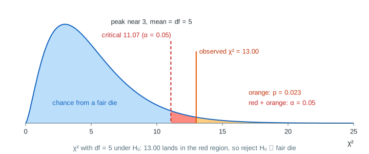
If H₀ is true, χ² follows (approximately) the chi-square distribution with df = k − 1 degrees of freedom, k being the number of categories. With 6 faces df = 5: the counts must add to 60, so once five are known the sixth is fixed. The curve starts at 0, peaks near 3 and has a long right tail; its mean is df = 5. It is the distribution of a sum of 5 squared standard normals, which is where the squares in the formula lead (each (O − E)/√E is close to normal by the central limit theorem).
p-value, α and the critical value
The p-value is P(χ² ≥ observed | H₀): the orange area right of the observed value. The test is one-tailed, because a bad fit can only make χ² larger. The significance level α fixes a critical value with right-tail area α; reject H₀ when χ² reaches it, which is the same as p ≤ α (Demo: α sets the critical value).
| α | critical value, df = 5 | 20 sixes (χ² = 13.00, p = 0.0234) |
|---|---|---|
| 0.10 | 9.236 | reject H₀ |
| 0.05 | 11.070 | reject H₀ |
| 0.01 | 15.086 | keep H₀ |
False alarms and power
A fair die still lands in the red tail sometimes. Those rejections are type I errors, and they happen about α of the time (Demo: false alarms with a fair die). A loaded die is caught only when its χ² lands past the critical value: with P(six) = 0.30 and 60 rolls that happens about half the time (Demo: power against a loaded die); with P(six) = 0.25 only about 1 in 5. The misses are type II errors. More rolls raise the power: the same bias makes χ² grow in proportion to n. The logic is the same as for one coin, see hypothesis testing with a coin.
When the test can be trusted, and other uses
- The chi-square curve is an approximation. The usual rule: every expected count E should be at least 5. With fewer rolls, merge categories or use an exact test.
- The categories must not overlap, and each roll counts once. Percentages are not counts: the test must use the raw numbers.
- The same Σ (O − E)²/E tests independence in a two-way table (does clicking depend on which page version a user saw?), with E = row total × column total / grand total and df = (rows − 1)(columns − 1). A 2 × 2 table is the chi-square version of an A/B test.
- A χ² that is far too small (counts suspiciously close to E) can also be a warning sign of made-up data, but the standard test does not reject for it.
What the page leaves out
- Unequal expected probabilities (H₀ such as 9 : 3 : 3 : 1 for Mendel's peas); the formula is the same with E = n × pᵢ.
- Fitting parameters from the data first, which removes one more degree of freedom per parameter.
- Exact multinomial tests, the G-test (likelihood ratio), Fisher's exact test and Yates' continuity correction for 2 × 2 tables.
- Effect sizes such as Cramér's V, and which faces caused the rejection (standardised residuals).