The idea: one coin, two questions
You flip a coin 10 times and get 7 heads. What is its heads probability p? Two schools of statistics answer with the same arithmetic but different meanings. The frequentist says p is a fixed number we don't know; only the data is random. The Bayesian says we are unsure about p, so p gets a probability distribution, and the data updates it.
The canvas runs both on the same flips. The strip at the top holds the flips; the FREQUENTIST panel and the BAYESIAN panel each turn them into an estimate and a 95% interval. The orange line is the true p. You can see it; neither method can.
The likelihood, shared by both
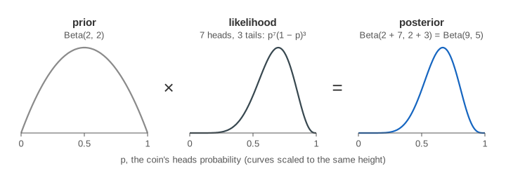
For a guess p, the chance of the exact sequence seen is the likelihood L(p) = ph(1 − p)t, with h heads and t tails. Each head multiplies it by p, each tail by 1 − p, so the curve changes one factor per flip (Demo: flip by flip, both curves narrow). The likelihood is not a probability distribution over p: its area is not 1, so the page scales its peak to the top of the plot and calls it relative.
Frequentist: estimate and confidence interval
The maximum likelihood estimate is the p where the likelihood peaks: p̂ = h/n = 7/10 = 0.70. The 95% confidence interval is a recipe that turns any data set into an interval. The page uses the Wilson score interval; the textbook Wald interval p̂ ± 1.96·√(p̂(1 − p̂)/n) shrinks to a single point after 3 heads in 3 flips. For 7 of 10 it gives [0.40, 0.89]. The p-value for H₀: p = 0.5 is 0.344, so a test would not call the coin biased (see Hypothesis Testing with a Coin).
With no flips the frequentist has nothing to say: no estimate and no interval. With 3 heads in 3 flips it says p̂ = 1.00, a coin that never lands tails (Demo: 3 heads in 3 flips).
Bayesian: prior to posterior, flip by flip
The Bayesian starts from a prior, a distribution for p before any flip. The Beta(a, b) family is handy for coins: multiply Beta(a, b) by ph(1 − p)t and you get Beta(a + h, b + t). So the posterior is just a counter: a counts heads, b counts tails, and the prior acts like a + b − 2 imaginary flips (see Bayes' Theorem for the rule itself).
| prior | like having already seen | after 7 of 10: posterior | mean |
|---|---|---|---|
| flat Beta(1, 1) | nothing | Beta(8, 4) | 0.67 |
| mild Beta(2, 2) | 1 head, 1 tail | Beta(9, 5) | 0.64 |
| strong Beta(20, 20) | 19 heads, 19 tails | Beta(27, 23) | 0.54 |
The 95% credible interval cuts 2.5% of the posterior's area off each end; the shaded blue area under the curve is the 95%. For 7 of 10 with a flat prior it is [0.39, 0.89], almost the same numbers as the confidence interval. The posterior also answers questions a confidence interval can't, such as P(p > 0.5 | flips) = 0.887.
What each 95% statement means
The numbers can match while the claims differ. The confidence interval's 95% is about the recipe: run the experiment again and again, and 95% of the intervals it makes contain the fixed p. Any single interval either contains p or doesn't. The credible interval's 95% is about p: given the prior and these flips, p is in this interval with probability 0.95.
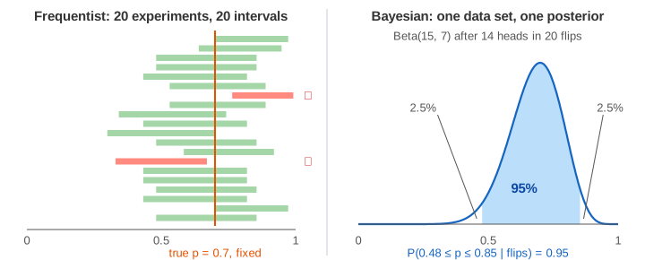
Press Repeat 20× to see it (Demo: what 95% means: 20 repeats): 20 fresh experiments with the same n, one row per experiment, green ✓ when the interval contains the true p and red ✗ when it misses. Confidence Intervals shows the same idea for a mean.
When they agree and when they don't
| situation | frequentist | Bayesian |
|---|---|---|
| no flips | no answer | the prior is the answer |
| 3 heads in 3 flips | p̂ = 1.00, CI [0.44, 1.00] | flat: mean 0.80, [0.40, 0.99]; mild: mean 0.71 |
| 14 heads in 20, strong prior | p̂ = 0.70, CI [0.48, 0.85] | mean 0.57, [0.44, 0.69]: pulled toward 0.5 |
| 100 flips | almost the same interval: the data outweighs any reasonable prior | |
| wrong strong prior, coin p = 0.9 | about 95% of CIs contain p | most credible intervals miss p |
With little data the prior matters and keeps the Bayesian away from extreme answers like p̂ = 1 (Demo: a strong prior pulls toward 0.5). With a lot of data the two meet (Demo: 100 flips, the two agree). The price of a prior is that a confident wrong one stays wrong for a while (Demo: a wrong strong prior misses): the credible interval is only as good as the prior you feed it.
What the page leaves out
Only one parameter and one conjugate prior family. Real Bayesian models have many parameters and usually need sampling (MCMC) instead of a closed-form posterior; the Jeffreys prior Beta(½, ½), highest-density intervals, Bayes factors, the exact Clopper–Pearson interval and the debate over stopping rules are not shown.