The idea: one number for "how close to a straight line"
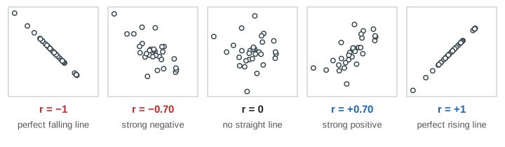
A scatter plot draws each pair (x, y) as one dot: hours studied and exam score, TV hours and score, time and height. The Pearson correlation coefficient r sums the picture up in one number from −1 to +1. Near +1 the dots lie close to a rising line, near −1 close to a falling line, and near 0 there is no straight-line pattern. r says how straight the pattern is, not how steep it is and not why it is there.
Quadrants and products
First find the mean point (x̄, ȳ). Its two lines split the plot into four quadrants. For each point multiply its two distances from the means: (x − x̄)(y − ȳ). A point up-right (both distances positive) or down-left (both negative) gives a positive product. A point up-left or down-right gives a negative one. On the canvas each product is a rectangle from the mean point to the dot: blue for positive, red for negative. Their total, Sxy = Σ (x − x̄)(y − ȳ), is the blue area minus the red area (Demo: study hours vs score).
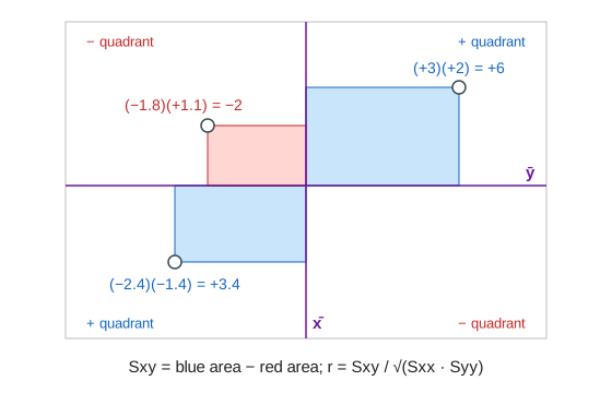
When most points sit in the blue quadrants, Sxy is large and positive. When most sit in the red ones, it is negative (Demo: TV hours vs score). When they are spread over all four, the areas cancel and Sxy is near 0.
Why divide by √(Sxx · Syy)
Sxy depends on units: measure study time in minutes instead of hours and Sxy grows 60 times. To remove the units, divide by the same kind of sum for each variable alone, Sxx = Σ (x − x̄)² and Syy = Σ (y − ȳ)²:
r = Sxy / √(Sxx · Syy)
By the Cauchy–Schwarz inequality the result is always between −1 and +1, and it is ±1 only when every point is exactly on one line. r does not change if you rescale or shift x or y, and it is the same if you swap x and y. Rough words for |r|: below 0.1 none, up to 0.4 weak, up to 0.7 moderate, above 0.7 strong. These cut-offs are habits, not laws.
One outlier can fake or wreck r
r adds up products, and a point far from the mean gives a huge rectangle. Shoe size and exam score have no relation (r ≈ 0). Add one typing error, shoe size 52 and score 92, and its single blue rectangle outweighs all the others: r jumps to a "moderate" value (Demo: no relation, then one outlier). It works the other way too: one student who was ill on the exam day drops study hours vs score from 0.91 to about 0.48. Toggle Outlier on any data set to see the grey "before" mark on the gauge. Always look at the scatter plot before you trust r.
A perfect curve can have r = 0
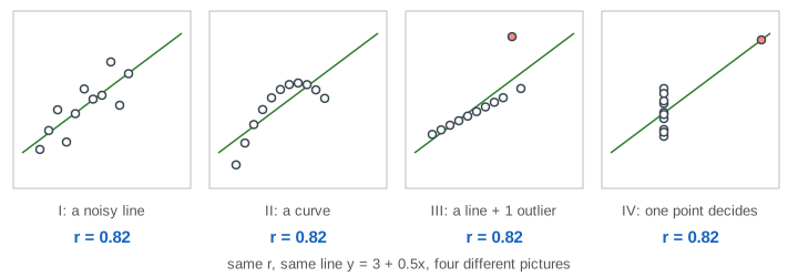
A ball thrown up follows h = 20t − 5t². Height is an exact function of time, yet r = 0: the rising half of the flight gives blue rectangles, the falling half gives mirror-image red ones, and they cancel (Demo: a thrown ball). r = 0 means "no straight-line relation", not "no relation". Anscombe's quartet makes the same point: four data sets with the same means, the same r and the same fitted line, and four very different pictures.
Correlation is not causation
Ice cream sales and sunburn cases rise and fall together, r ≈ 0.95 (Demo: ice cream and sunburns). Ice cream does not cause sunburn: hot, sunny days drive both. A hidden variable that moves both x and y is a confounder. A strong r can also come from y causing x (reverse causation), from chance in a small sample, or from looking at many pairs and reporting the best one. Showing cause needs a controlled experiment, or careful methods that adjust for confounders.
r and the regression line
The last step draws the least-squares line. It passes through (x̄, ȳ) with slope b = Sxy / Sxx = r · sy / sx, so r and the slope always have the same sign. r² is the share of the spread in y that the line explains: r = 0.9 gives r² = 0.81, so 81%. How the line is found is on Linear & Logistic Regression and Least Squares as Projection.
See also Mean vs Median vs Mode, where one outlier drags the mean just as it drags r here, and Hypothesis Testing with a Coin, the idea behind asking whether an r from a small sample could be chance.
What the page leaves out
Significance tests and confidence intervals for r (the t-test with n − 2 degrees of freedom, Fisher's z), covariance itself (Sxy / (n − 1)), rank correlations that handle curves that only rise (Spearman's ρ, Kendall's τ), robust alternatives that resist outliers, partial correlation that removes a known confounder, correlation matrices for many variables, and distance correlation or mutual information, which do detect curved relations like the ball's.
See where this page fits on the Probability & Statistics mind map.