The idea: two questions about more processors
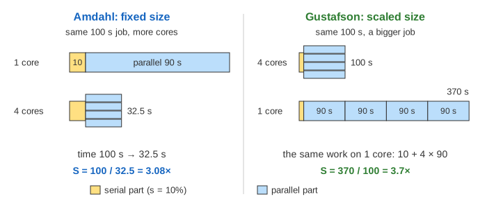
Every program has a serial part that only one processor can run (reading input, setting up, combining results) and a parallel part that can be split. Call the serial share s. There are two ways to ask what N processors buy you. Amdahl's law keeps the job fixed and asks how much faster it finishes. Gustafson's law keeps the time fixed and asks how much more work gets done.
The page uses the simplest model: the parallel part splits evenly, and starting threads, sending data and waiting on locks cost nothing. Real programs do worse.
Amdahl's law: fixed size
Take a job that runs 100 s on 1 core, with s = 10 %: 10 s serial and 90 s parallel. On N cores the serial 10 s stays, and the 90 s becomes 90 / N. So the time is T(N) = 10 + 90 / N, and the speedup is S = 100 / T. In general:
On 1, 2, 4 and 8 cores the job takes 100, 55, 32.5 and 21.25 s: speedups 1, 1.82, 3.08 and 4.71 (Demo 1). Even with endless cores the time never drops below the 10 s serial part, so the speedup can never pass 1 / s = 10×. This kind of test, one fixed job on more processors, is called strong scaling.
Where the curve flattens
The Amdahl curve rises fast at first and then bends flat. A handy point: it reaches half of its limit at N = (1 − s) / s. With s = 10 % that is 9 cores for 5×. The next 55 cores, up to 64, add less than 4× more: 16, 32 and 64 cores give 6.40, 7.80 and 8.77 (Demo 2). At 64 cores the serial 10 s is 88 % of the 11.41 s run.
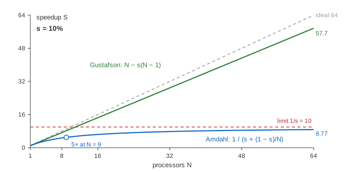
A bigger serial part flattens the curve sooner. With s = 25 % the limit is 4×, half of it comes at N = 3, and 4, 16 and 64 cores give 2.29, 3.37 and 3.82 (Demo 5). So Amdahl's law says: before buying more cores, make the serial part smaller.
Efficiency
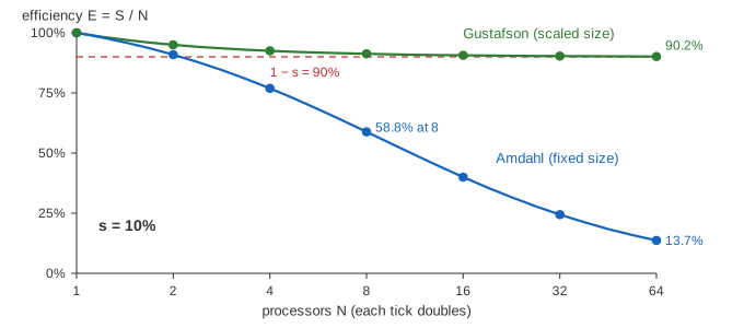
Efficiency E = S / N is the share of the cores' time that does useful work. 100 % means every core was busy all the time. Under Amdahl's law it falls as N grows, because N − 1 cores sit idle during the serial part.
| N | Amdahl S (s = 10 %) | Amdahl E | Gustafson S (s = 10 %) | Gustafson E |
|---|---|---|---|---|
| 2 | 1.82 | 90.9 % | 1.90 | 95.0 % |
| 8 | 4.71 | 58.8 % | 7.30 | 91.3 % |
| 16 | 6.40 | 40.0 % | 14.50 | 90.6 % |
| 64 | 8.77 | 13.7 % | 57.70 | 90.2 % |
Gustafson's law: scaled size
In 1988 John Gustafson pointed out that people with more processors usually run bigger problems: finer grids, more pixels, more data. So keep the run time fixed. On N cores the job takes 100 s: 10 s serial, then 90 s of work on every core. The same job on 1 core would take 10 + N × 90 s. On 8 cores that is 730 s, so the scaled speedup is 730 / 100 = 7.3 (Demo 3). In general, with s measured on the parallel run:
This is a straight line just under the ideal S = N. On 64 cores Amdahl gives 8.77× while Gustafson gives 57.7× for the same s = 10 % (Demo 4). Testing with the work per processor held fixed is called weak scaling.
Same run, two views
The two laws do not disagree. They fix different things, and their s comes from different runs. Gustafson's s = 10 % is measured on the 8-core run. Put the grown 730 s job on 1 core and its serial part is only 10 / 730 = 1.4 %. Amdahl's law with s = 1.4 % and N = 8 gives 7.30×, the same number (Demo 6). The lesson: when the serial part stays small while the job grows, more processors keep paying off.
| Amdahl | Gustafson | |
|---|---|---|
| What stays fixed | The job (problem size) | The time (work per processor) |
| Where s is measured | On 1 processor | On N processors |
| Speedup | 1 / (s + (1 − s) / N), at most 1 / s | N − s(N − 1), grows without limit |
| Efficiency as N grows | Falls towards 0 | Levels off at 1 − s |
| Test name | Strong scaling | Weak scaling |
| Fits | A fixed task you want done sooner: one build, one query | Science and data jobs that grow with the machine |
See also Parallel hardware: SIMD, multithreading and multicore for the cores themselves, Concurrency vs Parallelism for a fork–join program whose serial part caps it at 4×, the Java ForkJoinPool for splitting work over threads, a PostgreSQL parallel query for the serial gather step in a real engine, and MapReduce for a job that scales with the data.
See also MPI: Send, Receive and Collectives, where a parallel sum on 8 ranks spends one round on real work and six rounds moving data.
See also OpenMP loop scheduling, which shows how load imbalance leaves threads idle at the barrier and lowers the efficiency of a parallel loop.
See also Parallel Prefix Sum, which counts work and span for three scan algorithms and shows why extra work costs time when processors are few.
What the page leaves out
The model has no overhead: real runs pay to start threads, send data, synchronize and balance the load, and that cost often grows with N, so real speedup can even go down past some N. Superlinear speedup (S > N, when the data starts fitting in the caches) is left out. So are the Karp–Flatt metric for measuring s from real timings, the isoefficiency function, memory-bound limits and Sun–Ni's memory-bounded speedup.