The idea: running totals without waiting for the one before
A prefix sum, also called a scan, turns a list into its running totals. For x = 3 1 7 0 4 1 6 3 the inclusive scan is 3 4 11 11 15 16 22 25: cell i holds x[0] + … + x[i]. The exclusive scan is 0 3 4 11 11 15 16 22: cell i holds the sum of everything before i. The loop x[i] = x[i − 1] + x[i] does only 7 additions, but each one needs the result of the one before it. That chain is 7 steps long, and no number of processors can shorten it (Demo 1). The parallel algorithms on this page add the numbers in a different order, so that many additions can run at the same time.
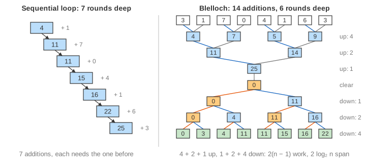
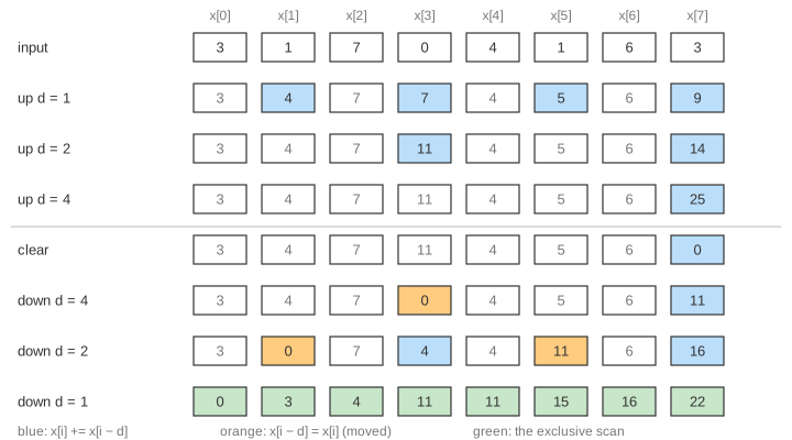
On the canvas each row is the shared array after one round, with time going down. A blue line goes from a value that is added, an orange line from a value that is moved, and a grey line from a cell to itself. Grey numbers were only copied in that round. The results table on the right keeps one row per algorithm, so you can compare them.
The PRAM, work and span
A PRAM (parallel random-access machine) is the textbook model: p processors share one memory and run in lock-step rounds. In a round every processor reads, computes and writes once. Two numbers describe an algorithm on it:
- Work W: the operations in total. It is the time on one processor.
- Span S (or depth): the number of rounds when processors are unlimited. It is the longest chain of operations that depend on each other.
An algorithm is work-efficient if its work is of the same order as the best sequential algorithm, here O(n). With p processors, a round of k operations takes ⌈k / p⌉ time steps. Adding that up gives Brent's bound: Tp ≤ W / p + S. The page uses the processor counts p = 8 (one per element) and p = 2.
Hillis–Steele: few rounds, more work
In round d = 1, 2, 4, every i ≥ d adds x[i − d]. After round d each cell holds the sum of the last 2d values, so after log₂ 8 = 3 rounds it holds everything (Demo 2). The rows are 3 4 8 7 4 5 7 9, then 3 4 11 11 12 12 11 14, then 3 4 11 11 15 16 22 25. Every processor reads its cell and a cell to its left, which another processor is writing, so a real machine needs a second buffer: the new row. The price is work. Round d does n − d additions: 7 + 6 + 4 = 17, against 7 for the loop.
| n | sequential work = span | Hillis–Steele work | span | Blelloch work | span |
|---|---|---|---|---|---|
| 8 | 7 | 17 | 3 | 14 | 6 |
| 1024 | 1023 | 9217 | 10 | 2046 | 20 |
| 220 ≈ 106 | 1048575 | 19922945 | 20 | 2097150 | 40 |
Hillis–Steele's work is n log₂ n − (n − 1). At a million values that is 19 times the loop's work, so it pays only when there are about as many processors as values, as inside one GPU warp.
Blelloch: up-sweep and down-sweep
Blelloch's scan works on a balanced binary tree laid over the array, without building the tree: the tree nodes are array cells.
- Up-sweep (a reduction): at distance d = 1, 2, 4, the right cell of each block of 2d adds the left half's total. 4 + 2 + 1 = 7 additions. The rows are 3 4 7 7 4 5 6 9, then 3 4 7 11 4 5 6 14, then x[7] = 25, the total.
- Clear: x[7] = 0, one write.
- Down-sweep: at d = 4, 2, 1, each pair (i − d, i) does
t = x[i − d]; x[i − d] = x[i]; x[i] += t. The left child gets the parent's value, which is the sum of everything to its left. The right child gets that plus the left subtree's total. 1 + 2 + 4 = 7 additions.
The result is the exclusive scan 0 3 4 11 11 15 16 22 after 14 = 2(n − 1) additions in 2 log₂ n = 6 rounds (Demo 3). It does twice the loop's work, which is still O(n), so it is work-efficient. If you need the inclusive scan, add x[i] to each cell: one more round.
With only two processors
Span counts rounds as if processors were free. With p = 2 every round of k additions takes ⌈k / 2⌉ time steps (Demo 5):
| algorithm | work | rounds | steps, p = 8 | steps, p = 2 |
|---|---|---|---|---|
| sequential | 7 | 7 | 7 | 7 |
| Hillis–Steele | 17 | 3 | 3 | 4 + 3 + 2 = 9 |
| Blelloch | 14 | 6 | 6 | 2 + 1 + 1 + 1 + 1 + 2 = 8 |
With 8 processors Hillis–Steele is fastest (Demo 4). With 2, the extra work shows: Blelloch beats it, and on only 8 values both lose to the plain loop. Real libraries therefore use a blocked scan: each of p processors scans its own block of n / p values with the loop, the p block totals are scanned (with Blelloch when p is large), and each block adds its offset. That does about 2n work in about 2n / p + log p time.
A use: stream compaction
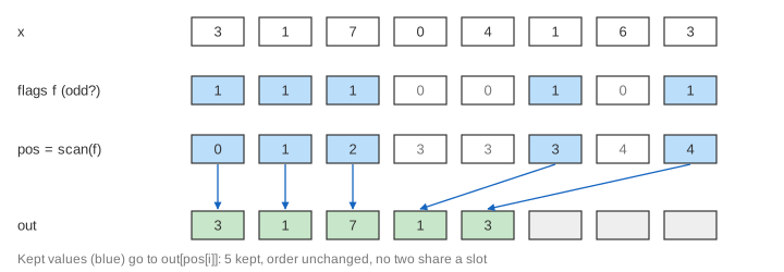
Scan answers the question "where does my value go?" in parallel. To keep only the odd values of 3 1 7 0 4 1 6 3 (Demo 6):
- Each processor sets a flag: f = 1 1 1 0 0 1 0 1. One round, 8 tests.
- An exclusive scan of the flags gives pos = 0 1 2 3 3 3 4 4: each kept value's slot is the number of kept values before it. 14 additions in 6 rounds.
- Each kept value writes itself to out[pos[i]]: out = 3 1 7 1 3. No two values share a slot, so no locks are needed. One round, 5 writes.
That is 27 operations in 8 rounds. The count is pos[7] + f[7] = 5. The same pattern splits values in radix sort on GPUs, where counting sort's running totals of the counts are a scan too.
A tree reduction is the up-sweep alone; on distributed memory it is MPI_Reduce on a binomial tree, and MPI also has MPI_Scan. How much speedup the parallel rounds buy for a whole program is the subject of Amdahl's and Gustafson's laws. On a GPU, 32 threads of a warp run in lock-step much like a PRAM. When the array changes and prefix sums are asked again and again on one processor, a Fenwick tree or a segment tree answers each in O(log n).
See also OpenMP loop scheduling for how a parallel for splits a loop over threads with static, dynamic and guided schedules.
What the page leaves out
The page uses n = 8, a power of two; other sizes pad the array or stop the tree early. Real GPU scans (CUB, Thrust) run a blocked scan per thread block and pass block totals with "decoupled look-back" in a single pass over memory, and they avoid shared-memory bank conflicts by padding. Left out: other associative operators (max, logical or, matrix product) that scan works for; segmented scan; carry-lookahead adders, which are a scan in hardware; Kogge–Stone, Brent–Kung and Ladner–Fischer networks; the CREW vs EREW details; and memory traffic, which matters more than additions on real machines. Floating-point sums can differ slightly between the algorithms because they add in a different order.