The idea: the same factor in every layer
Before a network learns anything, its weights are random numbers. How big those numbers are decides whether a signal can even get through the network. Each layer multiplies the spread of its input by about the same factor. Below 1, the signal shrinks a little more in every layer and vanishes. Above 1, it explodes. Ten layers with a factor of 8 give 8¹⁰ ≈ 10⁹. A good weight initialization picks the size of the random weights so the factor is about 1.
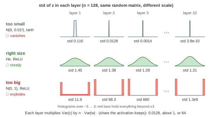
The page computes a real network in your browser: 10 fully connected layers of n = 128 units, no bias, and a batch of 64 inputs drawn from N(0, 1). Every init scheme scales the same random matrix, so only the scale differs. The top panel shows a histogram of the pre-activation z = a·W in each layer. The chart below it shows the standard deviation of z (blue) and of the gradient δ = ∂L/∂z (orange) on a log scale.
Why there is a factor: Var(z) = n · Var(w) · E[a²]
One unit adds up n products: z = w₁a₁ + w₂a₂ + … + wₙaₙ. The weights are independent, with mean 0. The variance of a sum of independent terms is the sum of their variances, so
Var(z) = n · Var(w) · E[a²]
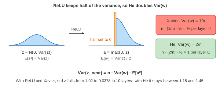
E[a²] is the mean square of the previous layer's outputs. The activation decides how much of Var(z) survives into E[a²]. A small z passes through tanh almost unchanged, so E[a²] ≈ Var(z). ReLU sets the negative half to 0, so E[a²] = Var(z) / 2. Each layer therefore multiplies Var(z) by n · Var(w) for tanh, or by n · Var(w) / 2 for ReLU. The page prints this sum with the measured numbers at every layer, next to the measured std.
Vanishing, exploding and saturation
| init (n = 128) | activation | factor on Var(z) | std z: layer 1 → 10 | what happens |
|---|---|---|---|---|
| N(0, 1) | ReLU | 128 / 2 = 64 | 11.6 → 1.3e9 | ✗ explodes, ×7.8 per layer |
| N(0, 0.01²) | tanh | 0.0128 | 0.116 → 3.8e-10 | ✗ vanishes, ×0.11 per layer |
| N(0, 1) | tanh | 128, capped by tanh | 11.6 → 11.0 | ✗ saturated: 85 % of units at |z| > 2 |
| Xavier | tanh | 1 | 1.02 → 0.258 | ✓ slow drift |
| He | ReLU | 1 | 1.45 → 1.21 | ✓ steady |
With ReLU and N(0, 1) weights the std of z is 1.3 × 10⁹ at layer 10; from layer 6 on, typical values are beyond float16's largest number, 65504 (Demo: N(0, 1) with ReLU — activations explode). With tiny weights, std z is 3.8 × 10⁻¹⁰ at layer 10: every input gives the same output, so the network has forgotten its input (Demo: N(0, 0.01²) with tanh — the signal vanishes).
tanh cannot explode, because its output stays between −1 and 1. Big weights cause a different failure: saturation. When |z| > 2, tanh is flat (tanh′(2) = 0.07), so the unit's output is just the sign of z. With N(0, 1) weights, 85 % of the units in every layer are there. The histograms pile up in the red end bins (Demo: N(0, 1) with tanh — every unit saturates).
Xavier / Glorot initialization
Glorot and Bengio (2010) chose Var(w) = 2 / (n_in + n_out). With equal widths that is 1/n, so the factor n · Var(w) is 1 for an activation that acts like the identity near 0, such as tanh. The average of n_in and n_out is a compromise between the forward pass (which needs n_in · Var(w) = 1) and the backward pass (which needs n_out · Var(w) = 1). In the page, std z drifts slowly from 1.02 to 0.258, because tanh squeezes large values a bit (Demo: Xavier with tanh — steady).
He / Kaiming initialization
ReLU throws away half of the variance, so Xavier with ReLU halves Var(z) in every layer: std z falls from 1.02 to 0.0378, ×0.69 per layer. He et al. (2015) doubled the weights' variance to make up for it: Var(w) = 2 / n_in. Then the factor is n · (2/n) / 2 = 1, and std z stays between 1.15 and 1.45 across all 10 layers (Demo: ReLU — Xavier shrinks, He stays steady). The dark marks on the chart keep the previous run, so you can compare the two.
| scheme | Var(w) | σ at n = 128 | made for | PyTorch |
|---|---|---|---|---|
| Xavier / Glorot | 2 / (n_in + n_out) | 0.0884 | tanh, sigmoid, linear | nn.init.xavier_normal_ |
| He / Kaiming | 2 / n_in | 0.125 | ReLU and its relatives | nn.init.kaiming_normal_ |
The backward pass has the same factor
Backpropagation sends the gradient back through the same weights: δ = (δ_next · Wᵀ) ⊙ f′(z). So Var(δ) is multiplied by n · Var(w) · E[f′(z)²] per layer, the mirror image of the forward pass. The page feeds a stand-in gradient drawn from N(0, 1) into layer 10 and shows how big it is at each earlier layer. With tiny weights it is 1.00 at layer 10 and 3.2 × 10⁻⁹ at layer 1: the first layers get no learning signal. With He and ReLU it stays near 0.7 everywhere. Saturated tanh is a surprise: tanh′ is only about 0.05, but n · Var(w) = 128 is bigger, so the gradient grows going back, from 0.217 to 676. Either way the layers learn at wildly different speeds. See Backpropagation for the chain rule step by step.
Wider layers, faster blow-up
The factor contains n. With N(0, 1) weights and ReLU, a layer of 32 units multiplies std z by about √(32/2) = 4, and a layer of 256 units by √(256/2) ≈ 11. After 10 layers that is 5.9 × 10⁵ against 5.7 × 10¹⁰ (Demo: wider layers explode faster with N(0, 1)). Xavier and He divide by n, so they work at any width; the Options group changes n.
In practice
PyTorch's nn.Linear starts with kaiming_uniform_(a=√5), a uniform distribution with
Var(w) = 1/(3·n_in), a little smaller than Xavier. Normalization layers (BatchNorm
and LayerNorm) and residual connections make deep networks much less sensitive to the init, but transformers
still scale the init of some layers by depth (GPT-2 divides the residual projections by √(2 · number of layers)).
The layers being initialized are the ones on Neural Network: the Forward Pass.
What the page leaves out
Biases (usually started at 0, as here), uniform instead of normal distributions (same variance, same behaviour), orthogonal initialization, LSUV, layers of different widths (where fan_in and fan_out differ), convolutions (where n is channels × kernel height × kernel width), the gain values for leaky ReLU and SELU, and what happens once training starts.