The idea: same formula, different axis
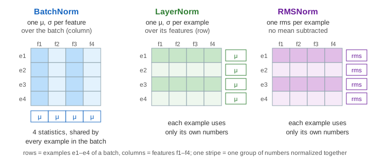
A layer in a neural network sees a batch: a table with one row per example and one column per feature. A normalization layer shifts and scales those numbers so they have a steady size, which keeps training stable. BatchNorm, LayerNorm and RMSNorm all use almost the same formula. The difference is which numbers they group together to compute the mean μ and spread σ. BatchNorm groups each column: one feature across all the examples in the batch. LayerNorm groups each row: one example across its own features. RMSNorm also works per row but only rescales.
The three formulas
For a group of numbers x, all three compute a normalized x̂ and then apply a learned scale γ and shift β: y = γ·x̂ + β. The page sets γ = 1 and β = 0 so you can see x̂ itself.
| group | x̂ | statistics kept | |
|---|---|---|---|
| BatchNorm | one feature, all B examples of the batch | (x − μ) / √(σ² + ε) | running μ and σ² per feature |
| LayerNorm | one example, all its features | (x − μ) / √(σ² + ε) | none |
| RMSNorm | one example, all its features | x / √(mean(x²) + ε) | none |
ε is a tiny number (10⁻⁵) that stops a division by zero. In a real network a feature is one of hundreds or thousands of channels; the page uses 4 features and up to 4 examples so every number fits on screen.
One batch, three answers
Batch A holds e1 = (2, 6, −1, 10), e2 = (4, 2, 1, 14), e3 = (9, 10, 11, 10) and e4 = (1, 2, −3, 6). BatchNorm's column means are μ = (4, 5, 2, 10) and σ = (3.08, 3.32, 5.39, 2.83), so e1 becomes (−0.65, 0.30, −0.56, 0.00): each value says how e1 compares with the other examples on that feature. LayerNorm uses e1's own μ = 4.25 and σ = 4.15 and gives (−0.54, 0.42, −1.27, 1.39): how each feature compares with e1's other features. RMSNorm divides by e1's rms = 5.94 and gives (0.34, 1.01, −0.17, 1.68). (Demo: one batch, three norms side by side)
e3 = (9, 10, 11, 10) shows the difference between LayerNorm and RMSNorm. LayerNorm removes its mean of 10 and gives (−1.41, 0, 1.41, 0). RMSNorm keeps the offset and gives (0.90, 1.00, 1.10, 1.00).
Your batchmates change your output
Batch B keeps e1 but replaces the other three with bigger numbers. BatchNorm's μ rises to (9.5, 12, 5, 17.5), and e1's output drops from (−0.65, 0.30, −0.56, 0.00) to (−1.65, −1.60, −1.60, −1.65): the same input, a different answer, only because of who else was in the batch. LayerNorm and RMSNorm give e1 exactly the same numbers as before. In training this noise acts a little like a regularizer; for anything else it is a problem. (Demo: same e1, new batchmates — only BatchNorm changes)
Small batches
BatchNorm needs enough examples to estimate each feature's mean and spread. With 2 examples every column comes out as exactly −1 and +1, whatever the values were. With 1 example each mean is the value itself, σ = 0 and every output is 0. PyTorch stops with “Expected more than 1 value per channel when training”. LayerNorm does not care: e1's row is the same for a batch of 4, 2 or 1. (Demo: small batches — 2 examples, then 1) This matters for big models, where one GPU may only fit a few long examples.
Training vs inference: running statistics
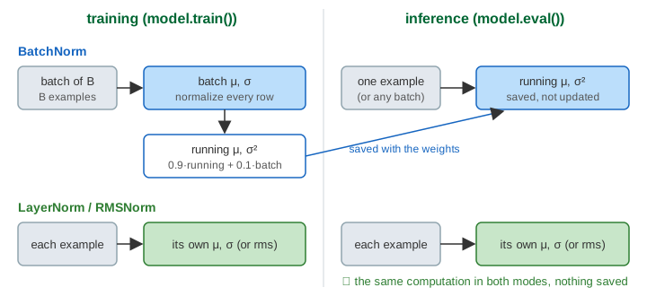
At inference a model often sees one example at a time, so BatchNorm cannot use batch statistics. During training
it keeps a running mean and running variance per feature, moved 10 % toward
each batch (momentum 0.1, starting at μ = 0, σ² = 1). model.eval() switches it to those saved
values. LayerNorm and RMSNorm keep nothing and compute the same thing in both modes.
Before any training the running statistics are still (0, 1), so at inference e1 comes out unchanged as
(2, 6, −1, 10). After 30 training batches the running μ is (3.62, 4.77, 0.01, 9.69), near the data's real means
(4, 5, 2, 10), and e1 comes out as (−0.63, 0.44, −0.19, 0.10). Forgetting model.eval(), or evaluating
on data whose statistics differ from training, are classic BatchNorm bugs.
(Demo: inference — running statistics before and after training)
Why transformers use LayerNorm or RMSNorm
A transformer's activations have the shape batch × tokens × features. Sentences have different lengths, so batches are padded, and at generation time the model produces one token at a time for one user. Statistics over the batch would mix sentences, count padding and change between training and generation. LayerNorm normalizes each token's feature vector on its own, so none of that matters. It sits around every self-attention and MLP block (before them in “pre-LN” models such as GPT-2 onward). Llama, Mistral and many newer models use RMSNorm: it skips the mean and the β shift, saves a little compute, and trains just as well. CNNs for images still often use BatchNorm, where batches are large and every image has the same shape.
| BatchNorm | LayerNorm | RMSNorm | |
|---|---|---|---|
| depends on other examples | yes (training) | no | no |
| batch of 1 | ✗ fails in training | ✓ | ✓ |
| train ≠ inference | yes, running stats | no | no |
| subtracts the mean | yes | yes | no |
| typical use | CNNs (ResNet) | transformers (BERT, GPT-2) | LLMs (Llama, Mistral) |
BatchNorm's training-time behaviour and its pairing with dropout are shown step by step on Dropout and Batch Normalization; the layers being normalized are the ones on Neural Network: the Forward Pass.
What the page leaves out
Real layers learn γ and β per feature; the page fixes them at 1 and 0. BatchNorm in a CNN takes its statistics over the batch and every pixel position of a channel, not just the batch. The page also leaves out GroupNorm and InstanceNorm (statistics over groups of channels or one image), SyncBatchNorm across GPUs, folding BatchNorm into the previous layer's weights for fast inference, and the exact placement debates (pre-LN vs post-LN, QK-norm).