Runge–Kutta vs Euler: More Slopes per Step

The idea: read the slope more than once per step

A differential equation y′ = f(x, y) gives the slope of the solution at every point. Euler's method reads the slope once, at the start of a step, and follows it in a straight line. The curve bends while you walk, so that one slope is already out of date by the end of the step. Runge–Kutta methods read the slope at a few trial points inside the step and walk with a weighted average of them. The classic one, RK4, uses four slopes.

Euler: one slope

Euler's step is y_n+1 = y_n + h·k₁ with k₁ = f(x_n, y_n). For y′ = y from y(0) = 1 with h = 1, k₁ = 1 and the step lands at 2, while the true value is e ≈ 2.718. The slope field, step size and stability of Euler's method are on Euler's Method; this page compares it with methods that take more samples.

Midpoint RK2: a trial half step

The midpoint method first follows k₁ for half a step to a trial midpoint, reads the slope k₂ there, then goes back to the start and takes the whole step with k₂:

k₂ = f(x_n + h/2, y_n + (h/2)·k₁),   y_n+1 = y_n + h·k₂

For the example, k₂ = f(0.5, 1.5) = 1.5 and the step lands at 2.5. It is a two-stage Runge–Kutta method, like Heun's method on the Euler page.

RK4: four slopes, weights 1, 2, 2, 1

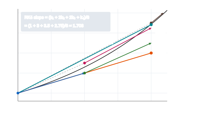
RK4 reads the slope at the start, twice at the midpoint, and at the end:

stage	read at	example (y′ = y, h = 1)	weight
k1	the start (xn, yn)	f(0, 1) = 1	1/6
k2	midpoint reached with k1: yn + (h/2)·k1	f(0.5, 1.5) = 1.5	2/6
k3	midpoint reached with k2: yn + (h/2)·k2	f(0.5, 1.75) = 1.75	2/6
k4	end point reached with k3: yn + h·k3	f(1, 2.75) = 2.75	1/6

y_n+1 = y_n + h·(k₁ + 2k₂ + 2k₃ + k₄)/6. Here the average slope is (1 + 3 + 3.5 + 2.75)/6 ≈ 1.708 and the step lands at 2.7083, an error of 0.01 after one big step. The weights 1, 4, 1 (the two midpoint slopes share the 4) are Simpson's rule: when f depends on x only, RK4 is exactly Simpson's rule for the integral (see Riemann sums). For y′ = y one RK4 step multiplies y by 1 + h + h²/2 + h³/6 + h⁴/24, the first five terms of the Taylor series of e^h. (Demo: one RK4 step on y′ = y, h = 1)

Order: halve h, divide the error by 2, 4 or 16

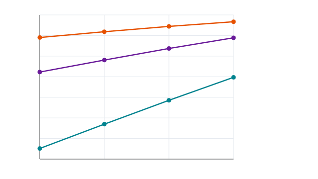
A method has order p when its global error at a fixed x is about C·h^p. Halving h then divides the error by 2^p. The error table on the canvas, for y′ = y at x = 1 (exact e ≈ 2.71828):

h	Euler error	ratio	RK2 error	ratio	RK4 error	ratio
0.5	0.468		0.0777		0.000936
0.25	0.277	1.7	0.0234	3.3	0.0000719	13.0
0.125	0.152	1.8	0.00644	3.6	0.00000498	14.4
0.0625	0.0804	1.9	0.00169	3.8	0.000000328	15.2

The ratios approach 2, 4 and 16: Euler is first order, the midpoint method second, RK4 fourth. RK4 with h = 0.5 (2 steps) is about 86 times more accurate than Euler with h = 0.0625 (16 steps). (Demo: error table, halve h)

Counting the work

The expensive part of a real solver is computing f (a force, a chemical rate, a whole simulation step). Euler costs 1 slope evaluation per step, RK2 costs 2 and RK4 costs 4. A fair comparison gives every method the same number of evaluations: RK4 with h = 0.5 against Euler with h = 0.125. Because the error falls like h⁴, RK4 still wins by far. The runs table on the canvas shows the evaluations of each run. (Demo: orbit, same work)

The orbit: Euler gains energy, RK4 does not

A mass on a spring, x″ = −x, is the system x′ = v, v′ = −x. Drawn with position x across and velocity v up (the phase plane), the exact motion from (1, 0) goes round the unit circle forever, because the energy E = (x² + v²)/2 never changes (the same motion as the spring oscillator and a circular orbit).

An Euler step moves along the tangent of the circle. The tangent leaves the circle on the outside, so each step multiplies the radius by √(1 + h²) and the energy by 1 + h². The errors never cancel: Euler spirals outward. With h = 0.25, one turn (25 steps) ends at radius 2.13 with 4.6 times the energy. RK4's radius factor is about 1 − h⁶/144: for h = 0.25 the radius after one turn is 0.99996.

one turn, from (1, 0)	h	steps	slope evaluations	radius (exact 1)	energy
Euler	0.25	25	25	2.134	✗ ×4.55
Midpoint RK2	0.25	25	50	1.012	×1.025
RK4	0.25	25	100	0.99996	✓ ×0.9999
Euler	0.125	50	50	1.473	✗ ×2.17
RK4	0.5	13	52	0.9986	✓ ×0.997

(Demo: orbit, Euler spirals outward; Demo: orbit, all three methods)

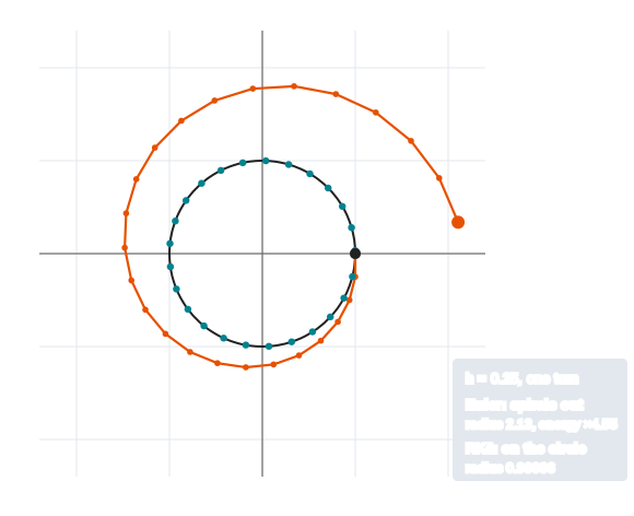
With friction added, the true orbit spirals inward instead; see Damped Oscillation. A numerical method that adds energy can hide that damping or invent motion that is not there, which is why the choice of method matters for long simulations.

RK4 with a fixed step dt = 0.01 traces a chaotic system on The Lorenz Attractor: Deterministic Chaos, where even the step size's tiny error grows until the path is different after t ≈ 20.

RK4 at work on a chaotic system, with the energy drift printed as a check of the integrator: The Double Pendulum: Normal Modes and Chaos.

What the page leaves out

RK4 also loses a little energy (radius factor just below 1), so over millions of steps it slowly spirals inward. For orbits, molecules and games, symplectic methods such as leapfrog / velocity Verlet are used: they are only second order but keep the energy bounded forever. Real solvers (RK45, Dormand–Prince, scipy.integrate.solve_ivp) pair two Runge–Kutta methods of different order to estimate each step's error and change h as they go. Stiff equations need implicit methods, and rounding error, which grows when h is extremely small, is ignored here.

References

Runge–Kutta methods (Wikipedia)

Midpoint method (Wikipedia)

Symplectic integrator (Wikipedia)

scipy.integrate.solve_ivp (SciPy documentation)