The idea: a pendulum hanging from a pendulum
Hang a second pendulum from the bob of the first and you get a double pendulum: a pivot, a rod, a bob, a second rod, a second bob. Nothing is random in it. Give it the same start twice and it does the same thing twice. Yet for big swings its motion is so irregular that a change of a millionth of a radian in the start makes a completely different motion a few seconds later. That is chaos.
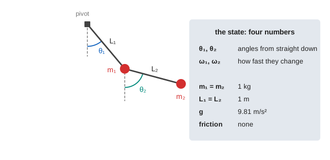
The page uses two equal bobs (m₁ = m₂ = 1 kg) on two equal rods (L₁ = L₂ = 1 m), g = 9.81 m/s², no friction. Both angles are measured from straight down, θ₁ at the pivot and θ₂ at the first bob.
The equations of motion
Write the kinetic energy KE and the potential energy PE of the two bobs, form the Lagrangian KE − PE, and Lagrange's equations give the two angular accelerations. With m = 1 kg and L = 1 m, and the short names Δ = θ₁ − θ₂ and D = 3 − cos 2Δ:
θ₁″ = (−3g sin θ₁ − g sin(θ₁ − 2θ₂) − 2 sin Δ·(ω₂² + ω₁² cos Δ)) / D
θ₂″ = 2 sin Δ·(2ω₁² + 2g cos θ₁ + ω₂² cos Δ) / D

KE = ω₁² + ½ω₂² + ω₁ω₂ cos Δ
PE = g·(3 − 2 cos θ₁ − cos θ₂)        (0 when it hangs straight down)
There is no formula for θ₁(t) and θ₂(t). A computer steps the equations forward in small time steps instead. The page uses the classic fourth-order Runge–Kutta method (RK4) with a fixed step dt = 1 ms, so 10 s of motion is 10 000 steps, and keeps a sample every 5 ms to draw. RK4 is the method from Runge–Kutta vs Euler.
Small swings: two normal modes
For small angles, sin θ ≈ θ and the products of small terms vanish. The equations become linear, and a linear system of two coupled pendulums has two normal modes: shapes that keep their form and swing at one frequency each.
| mode | shape | ω | period |
|---|---|---|---|
| in-phase | θ₂ = √2·θ₁: both bobs swing the same way | √((2 − √2)g/L) ≈ 2.40 rad/s | 2.62 s |
| anti-phase | θ₂ = −√2·θ₁: the bobs swing opposite ways | √((2 + √2)g/L) ≈ 5.79 rad/s | 1.09 s |
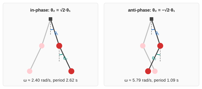
Start in a mode and the pendulum stays in it (Demo: in-phase normal mode, period 2.6 s and Demo: anti-phase normal mode, period 1.1 s): the trace is a single thin arc and the θ lines are two sine waves. At 10° the in-phase period is 2.63 s, close to the linear 2.62 s. The anti-phase swing bends the joint by 24°, which is no longer quite small, so it takes 1.14 s instead of 1.09 s.
Any other small start is a mix of the two modes. 10°, 10° is one (Demo: small swing, two modes mixed (10°, 10°)): the two periods do not fit a whole number of times into each other, so the motion is quasi-periodic: regular, but it never repeats exactly. In the angle chart the fast anti-phase wiggle rides on the slow in-phase swing. A single pendulum has just one mode: see Simple Pendulum.
Big swings: chaos
Give it more energy, 90°, 90° or 120°, −10° or 179°, 179°, and the sin terms stop being straight lines. The lower bob whips round, sometimes over the top, and the θ lines never settle into a pattern. The motion is chaotic: still fully determined by the start, but with sensitive dependence on initial conditions.
Choose 2, 10 or 50 pendulums: copy k starts with θ₂ larger by (k − 1)·10⁻⁶ rad, one hue each. At first they all sit on top of each other. Then the distance between copy 1 and copy 2 (the bottom chart, log scale) climbs along a rough straight line, which on a log scale means it grows exponentially: at 90°, 90° it goes from 2 × 10⁻⁵ at 10 s to 0.37 rad at 20 s, about tenfold every 2.4 s. Once the copies are a radian or so apart the line flattens out: they cannot get further apart than two unrelated states. (Demo: 90°, 90°: two copies 10⁻⁶ rad apart drift apart, Demo: rainbow fan-out, 50 copies at 179°, 179°.)
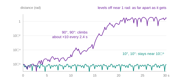
The growth rate is the Lyapunov exponent. Because errors grow this way, a start known to one part in a million is only good for a few seconds of prediction. The same thing limits weather forecasts: see the Lorenz Attractor, and the Logistic Map for chaos in a single line of arithmetic.
Energy as a check of the integrator
With no friction the total energy E = KE + PE cannot change. The middle chart shows KE (orange) and PE (green) trading places all the time while their sum (black) stays flat. The integrator does not know about this law, so watching E is a free test of how accurate it is. The "drift" line under the pendulum prints E − E₀ as it is, not rounded away.
| start | E₀ | biggest |E − E₀| in 60 s, dt = 1 ms | with dt = 5 ms |
|---|---|---|---|
| 10°, 10° | 0.447 J | 5 × 10⁻¹³ J | 1 × 10⁻⁹ J |
| 90°, 90° | 29.43 J | 4 × 10⁻⁸ J | 1 × 10⁻⁴ J |
| 179°, 179° | 58.86 J | 5 × 10⁻⁷ J | 1 × 10⁻³ J |
RK4's error per unit time shrinks like dt⁴: five times the step gives roughly 5⁴ = 625 times the drift, and more where the bob moves fast. (Demo: energy check, 120°, −10° for 30 s.) A small drift does not mean the chaotic path is right, though: the tiny error of each step grows like any other small difference. Run 90°, 90° with dt = 1 ms and with dt = 2 ms and the two paths are 0.05 rad apart at 25 s and completely different by 30 s. What stays right is the kind of motion and its statistics, not the exact path.
What the page leaves out
Friction and air drag, unequal masses or rods, rods with mass (a compound pendulum), starts with the bobs moving, the derivation of the equations step by step, the Hamiltonian form, Poincaré sections that show which starts are chaotic, and computing the Lyapunov exponent properly. The page keeps 60 s of motion. Energy-preserving (symplectic) integrators, which keep E bounded for ever, are left out too.