The idea: guess the sizes, price every plan, keep the cheapest
SQL says what rows you want, not how to get them. The same query can read the whole table or jump through an index, and join two tables in several orders and by several methods. The query planner (also called the optimizer) picks one. PostgreSQL's planner is cost-based: it estimates how many rows each step returns, turns that into a cost, and keeps the cheapest plan. It never looks at the table while planning. All it has is the statistics that the last ANALYZE collected.
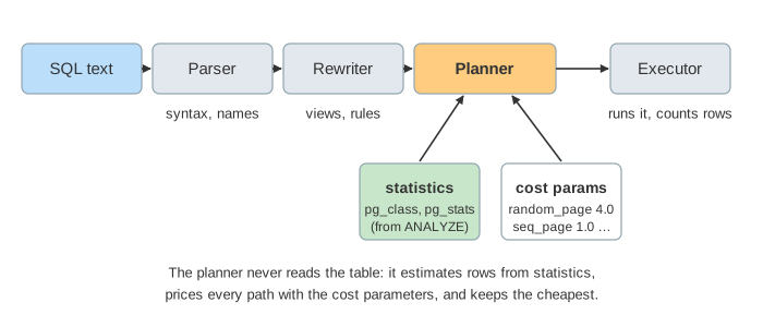
The page has two tables: orders (100 000 rows on 1 000 pages, indexes on id, status, customer_id and created_at) and customers (5 000 rows on 50 pages, primary key id). Pick a query and press EXPLAIN to watch it being planned, or EXPLAIN ANALYZE to plan it and run it. The change data or statistics select bulk-inserts rows, runs ANALYZE or creates extended statistics as soon as you pick an entry.
What the planner knows: statistics
ANALYZE (run by autovacuum, or by hand) reads a random sample of 300 × default_statistics_target = 30 000 rows and stores a summary per column:
| statistic | where | on this page | used for |
|---|---|---|---|
| rows and pages | pg_class.reltuples, relpages | orders 100 000 / 1 000 | table size, cost of reading it |
| most common values and their frequencies | pg_stats.most_common_vals, most_common_freqs | status: shipped 0.900, pending 0.080, cancelled 0.020 | col = value |
| histogram | histogram_bounds | created_at: 10 buckets of 10 % each | ranges, <, >= |
| number of distinct values | n_distinct | customer_id: 5 000; id: unique | equality on other values, joins |
| correlation | correlation | created_at: 1.0 (stored in date order) | how scattered an index scan's heap reads are |
The selectivity of a condition is the fraction of rows it keeps, and estimated rows = selectivity × reltuples. status = 'pending' is a most-common value with frequency 0.080, so 0.080 × 100 000 = 8 000 rows. created_at >= '2026-09-01' covers 1 of the 10 histogram buckets: 10 000 rows. id = 42 is unique: 1 row.
The cost model and the three scans
Costs are in arbitrary units where reading one page in order costs 1.0. The defaults:
| parameter | default | meaning |
|---|---|---|
seq_page_cost | 1.0 | read a page that comes next on disk |
random_page_cost | 4.0 | read a page somewhere else (lower it on SSDs, often 1.1) |
cpu_tuple_cost | 0.01 | process one row |
cpu_index_tuple_cost | 0.005 | process one index entry |
cpu_operator_cost | 0.0025 | evaluate one operator, such as status = 'pending' |
A Seq Scan reads every page in order and checks every row: 1 000 × 1.0 + 100 000 × (0.01 + 0.0025) = 2 250, whatever the WHERE. An Index Scan walks the index and fetches each matching row's page, a random read at 4.0. k random rows touch about T·(1 − e−k/T) of the T pages, so it is cheap for a few rows and very expensive for many. A Bitmap Heap Scan first collects all matching row ids from the index into a bitmap, then reads those pages once each and in page order, which costs less per page. It sits in between (Demo 2: selectivity picks the scan):
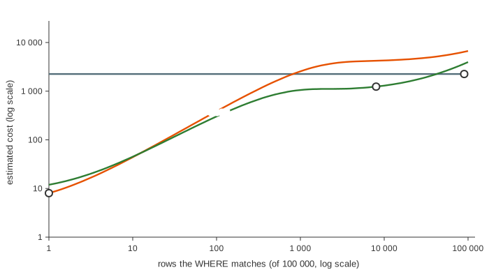
Correlation changes the picture. created_at is stored in date order, so the 10 000 matching rows sit on about 100 neighbouring pages and an Index Scan reads them almost sequentially: cost 373 instead of 4 000+ (Demo 3: range on an ordered column).
Join order and join method
For a join the planner first picks the cheapest scan for each table, then prices every way to combine them. It estimates the join's output as rows(orders) × rows(customers) / max(n_distinct) and tries both orders of the tables:
| method | how it works | good when |
|---|---|---|
| Nested Loop | for each outer row, look up matching inner rows (here through an index) | the outer side is a handful of rows (Demo 5: Q6, cost 16) |
| Hash Join | build a hash table from the smaller side, stream the other side through it | both sides are big and unsorted, equality join (Demo 4: Q5, cost 1 387) |
| Merge Join | sort both sides on the join key, walk them together | both inputs already come sorted, e.g. from an index, or the result must be sorted anyway |
With more tables the number of orders explodes. PostgreSQL searches them with dynamic programming up to geqo_threshold = 12 tables, and with a genetic algorithm above that. The JOIN, GROUP BY and ORDER BY page shows how the three join methods run.
Reading EXPLAIN and EXPLAIN ANALYZE
EXPLAIN prints the chosen plan as a tree: each line is a node, indented nodes feed the line above, and each has an estimated cost and rows. EXPLAIN ANALYZE also runs it and adds the real numbers:
Hash Join  (cost=… rows=800) (actual rows=800 loops=1)
  Hash Cond: (o.customer_id = c.id)
  ->  Bitmap Heap Scan on orders o  (cost=… rows=8000) (actual rows=8000 loops=1)
        Recheck Cond: (status = 'pending')
        ->  Bitmap Index Scan on orders_status_idx  (rows=8000) (actual rows=8000 loops=1)
  ->  Hash  (rows=500) (actual rows=500 loops=1)
        ->  Seq Scan on customers c  (rows=500) (actual rows=500 loops=1)
              Filter: (country = 'FR')
The first thing to check is estimated rows vs actual rows. When they differ by 10× or more (red on the canvas), the plan was chosen for the wrong size. On an inner node of a nested loop, rows is per loop: multiply by loops. The page shows the execution time as 0.02 ms per unit of actual work, so it is a simulation, not a measurement.
When statistics go stale
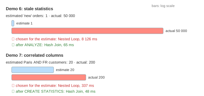
Statistics are only as fresh as the last ANALYZE. In Demo 6 a bulk import adds 50 000 orders with status 'new', a value the statistics have never seen. The planner clamps the estimate to 1 row and picks a Nested Loop: cost 16. In reality the index scan returns 50 000 rows and the loop does 50 000 lookups: about 8 100 ms. After ANALYZE the estimate is 50 000 and the planner picks a Hash Join: about 65 ms. Autovacuum runs ANALYZE when more than autovacuum_analyze_threshold (50) + autovacuum_analyze_scale_factor (10 %) of the rows changed, but not instantly. After a bulk load, run ANALYZE yourself.
Correlated columns and CREATE STATISTICS
For city = 'Paris' AND country = 'FR' the planner multiplies the two selectivities, as if the columns were independent: 0.040 × 0.100 × 5 000 = 20 rows. But every Paris customer is in France, so the truth is 200 (Demo 7). The 10× underestimate makes a Nested Loop look cheaper than a Hash Join. Extended statistics tell the planner that one column decides the other:
CREATE STATISTICS customers_city_country (dependencies) ON city, country FROM customers;
ANALYZE customers;
With the dependency (1.0) the estimate is 0.040 × 5 000 = 200 rows and the Hash Join wins. Other kinds are ndistinct (for GROUP BY on several columns) and mcv (common value combinations).
See also How PostgreSQL Runs a Query for what the executor does with heap pages, MVCC and WAL, and the B+ tree as a database index for what an index scan walks through. Database normalization shows where the joins come from: splitting a table to 3NF so each fact is stored once. The N+1 Query Problem shows the opposite mistake: many tiny queries from an ORM loop where one join would do.
An index-only scan avoids the heap only on all-visible pages; see PostgreSQL Free Space Map and Visibility Map. How a Bitmap Index Scan builds its TID bitmap, how BitmapAnd/BitmapOr combine two indexes and when pages go lossy is animated on PostgreSQL Bitmap Index Scan and Bitmap Heap Scan. Parallel plans (Gather over a Parallel Seq Scan) are animated in PostgreSQL parallel query.
For what MySQL's EXPLAIN type, key_len and Extra columns mean for each access path, see MySQL Index Access Paths and EXPLAIN.
See also Nested loop vs Hash join vs Merge join for when each join method is cheapest.
What the page leaves out
The real formulas in costsize.c (index correlation, effective_cache_size, startup vs total cost, parallel workers), the genetic optimizer, more than two tables, GROUP BY, ORDER BY and LIMIT (which change which plan is cheapest), Index Only Scans and the visibility map, BitmapAnd/BitmapOr of two indexes, prepared statements with generic plans, join hints, which PostgreSQL does not have, and real timing. The numbers come from one simplified cost model, so they are consistent with each other but are not what your server would print.