The idea: an arrow at every point, and curves that follow them
A linear system of two differential equations, x′ = ax + by and y′ = cx + dy, is written x′ = Ax with the matrix A = [[a, b], [c, d]] and the point x = (x, y). At every point of the plane it gives a velocity, the arrow Ax: that is the vector field. A solution is a curve that follows the arrows everywhere, a trajectory. Pick a starting point x(0) and the trajectory is fixed. All the trajectories drawn together form the phase portrait. The point (0, 0) never moves, since A·0 = 0: it is the fixed point (equilibrium), and the portrait shows what happens near it.
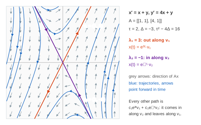
The canvas draws the arrows all the same length, so they show only the direction. Each trajectory is computed with RK4 steps of dt = 0.01, the method from Runge–Kutta vs Euler; it is the 2-D version of the slope field on Euler's method, where the field had one unknown y(t) and the arrows had slope f(t, y). Press Trace, or click the phase plane, to start one; Portrait traces eight starts both forward and backward in time.
Straight-line solutions from eigenvectors
Most trajectories curve. A few are straight lines through the origin. On such a line the arrow Ax must point along the line, so Ax = λx for a number λ: x is an eigenvector of A and λ its eigenvalue (see Eigenvectors & Eigenvalues). Then
x(t) = eλt·v
is a solution: it moves straight out along v when λ > 0 and straight in when λ < 0. With two independent eigenvectors every solution is a mix, x(t) = c₁eλ₁tv₁ + c₂eλ₂tv₂, and the larger exponent wins as t grows. For the saddle A = [[1, 1], [4, 1]] the eigenvalues are 3 and −1 with v₁ = (1, 2) and v₂ = (1, −2). A start on v₂'s line, such as (1.5, −3), slides straight into the origin. A start just beside it, (1.7, −3) = 0.1·v₁ + 1.6·v₂, first comes in but the small e3t part grows and it leaves along v₁. (Demo: saddle, eigenvectors are straight-line solutions)
Trace and determinant decide the picture
The eigenvalues solve det(A − λI) = λ² − τλ + Δ = 0, where τ = a + d is the trace and Δ = ad − bc the determinant:
λ = (τ ± √(τ² − 4Δ)) / 2, λ₁ + λ₂ = τ, λ₁·λ₂ = Δ
So two numbers sort every 2×2 system. The seven systems on the canvas:
| A | τ | Δ | τ² − 4Δ | λ | type |
|---|---|---|---|---|---|
| [[1, 1], [4, 1]] | 2 | −3 | 16 | 3, −1 | saddle: Δ < 0, real λ of opposite signs |
| [[−2, 1], [1, −2]] | −4 | 3 | 4 | −1, −3 | stable node: both λ < 0 |
| [[1, 1], [0, 2]] | 3 | 2 | 1 | 2, 1 | unstable node: both λ > 0 |
| [[−0.5, −2], [2, −0.5]] | −1 | 4.25 | −16 | −0.5 ± 2i | stable spiral |
| [[0.3, 1], [−2, 0.3]] | 0.6 | 2.09 | −8 | 0.3 ± 1.414i | unstable spiral |
| [[0, 1], [−4, 0]] | 0 | 4 | −16 | ±2i | centre |
| [[−1, 1], [0, −1]] | −2 | 1 | 0 | −1 (double) | degenerate node, one eigenvector |
In a node both eigenvalues have the same sign. Near the origin the paths line up with the slow eigenvector, the one with the smaller |λ|: for the stable node that is v₁ = (1, 1) with λ = −1, because the e−3t part along (1, −1) dies out first. (Demo: stable node, every path enters the origin; Demo: unstable node, paths leave the origin)
The trace–determinant plane
Put τ across and Δ up. The parabola τ² = 4Δ separates real eigenvalues (below it) from complex ones (above). The left half (τ < 0) is stable, the right half unstable, and everything under the τ axis (Δ < 0) is a saddle. The canvas moves a dot to the current A each time the system changes.
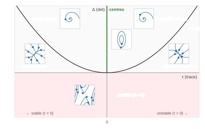
| where | eigenvalues | portrait |
|---|---|---|
| Δ < 0 | real, opposite signs | saddle: in along one eigenvector, out along the other ✗ unstable |
| 0 < Δ < τ²/4 | real, same sign as τ | node: ✓ stable if τ < 0 |
| Δ > τ²/4 | complex α ± iβ, α = τ/2 | spiral: ✓ stable if τ < 0 |
| τ = 0, Δ > 0 | ±iβ | centre: closed orbits, neither in nor out |
| Δ = τ²/4 | one repeated λ | degenerate (or star) node |
| Δ = 0 | one λ is 0 | a whole line of fixed points |
Complex eigenvalues: spirals and centres
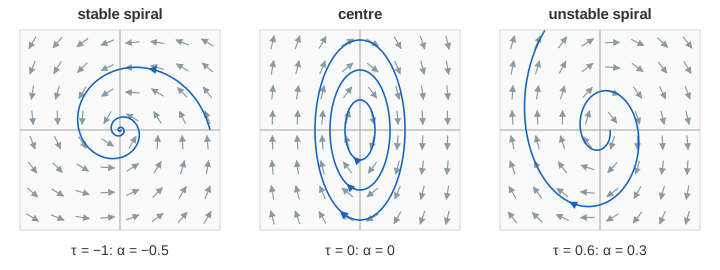
When τ² < 4Δ the eigenvalues are λ = α ± iβ with α = τ/2 and β = √(4Δ − τ²)/2. No real direction is mapped onto its own line, so there is no straight-line solution: the flow turns. The solutions are eαt times sines and cosines of βt, so one turn takes 2π/β and multiplies the distance to the origin by e2πα/β. The sign of c says which way: at (1, 0) the velocity is (a, c), so c > 0 turns counter-clockwise. For the stable spiral α = −0.5 and β = 2: each turn, taking π ≈ 3.14, shrinks the distance by e−π/2 ≈ 0.21. (Demo: spiral in vs spiral out)
With τ = 0 the shrinking stops. A = [[0, 1], [−4, 0]] is the spring x″ = −4x written as a system (y = x′); every orbit is the ellipse 4x² + y² = constant, closed after one period π (see Spring Oscillator). (Demo: centre, closed orbits). Slide τ from −0.5 through 0 to 0.5 with Δ fixed near 4 and the same matrix family goes from spiralling in, to closed orbits, to spiralling out: the dot crosses the positive Δ axis. (Demo: cross τ = 0, spiral in → centre → spiral out)
On the parabola: one eigenvector
A = [[−1, 1], [0, −1]] has τ² = 4Δ = 4 and a double eigenvalue λ = −1, but (A + I)v = 0 has only the solutions v = (s, 0). One eigenline, the x axis. The solution is e−t(x₀ + t·y₀, y₀): the extra t makes every path swing round and come in tangent to that single line. This borderline case sits between the nodes and the spirals. (Demo: degenerate node, only one eigenvector)
Why linear systems matter
Near a fixed point, a nonlinear system x′ = f(x) behaves like its linearisation x′ = Jx, where J is the matrix of partial derivatives at that point. Unless the linear part is a centre or lies on a borderline, the linear portrait tells you whether the fixed point attracts, repels or is a saddle. The fixed points C± of the Lorenz attractor are classified exactly this way, with a 3×3 matrix.
What the page leaves out
Only 2×2 constant matrices are shown, and only the window [−4, 4]². Higher-dimensional systems have more eigenvalues and mixed behaviours (a spiral in one plane, a saddle direction out of it). Nonlinear systems can have several fixed points, limit cycles and chaos, and their linearisation says nothing for centres. The exact solution eAtx₀ (the matrix exponential) and the generalised eigenvector of the degenerate case are only mentioned; the page integrates numerically instead.