Heat Equation Visualization | Finite Differences on a Rod

The idea: a cell moves toward the average of its neighbours

Heat flows from hot to cold. On a thin rod the temperature u(x, t) obeys the heat equation u_t = α·u_xx. The left side is how fast a point warms up. The right side is the curvature of the temperature profile, times the diffusivity α (about 1.1 cm²/s for copper). A point hotter than the average of its neighbours sits on a peak: u_xx < 0, so it cools. A point in a dip warms up. Peaks flatten, dips fill in, and every profile ends up smooth.

Temperature along a 16 cm rod with ends at 0 °C and r = 0.4: a 100 °C spike at 8 cm becomes 40, 20, 40 after one step, a low hump after 5 steps and a wide hump with peak 9.9 °C after 20 steps. Two rows of coloured cells show the values at n = 0 and n = 20 — One spike of heat spreads into a wide, low hump; the ends at 0 °C slowly drain it.

Finite differences, cell by cell

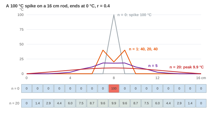
The page cuts the rod into cells Δx = 1 cm apart (17 grid points, 0 to 16 cm) and takes time steps of Δt. Replace the derivatives by differences: u_t ≈ (u_iⁿ⁺¹ − u_iⁿ)/Δt and u_xx ≈ (u_i−1 − 2u_i + u_i+1)/Δx². Solving for the new value gives the explicit scheme (FTCS, forward in time, centred in space):

u_iⁿ⁺¹ = u_iⁿ + r·(u_i−1ⁿ − 2u_iⁿ + u_i+1ⁿ), r = αΔt/Δx²

Read it as a weighted average: the new value is r·u_i−1 + (1 − 2r)·u_i + r·u_i+1. Every new value uses only the old row, which is why the canvas fills a second row uⁿ⁺¹ and copies it up when it is full. With α = 1 cm²/s and Δx = 1 cm, one step lasts Δt = r seconds. For the spike at r = 0.4, cell 8 becomes 100 + 0.4·(0 − 200 + 0) = 20 and cells 7 and 9 become 40. (Demo: a spike spreads, cell by cell; Demo: two bumps merge into one)

Stability: r ≤ 1/2

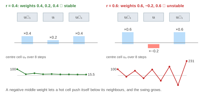
If r ≤ 1/2 all three weights are positive, so each new value lies between the old values around it: no new peaks, no temperatures below the coldest cell (a discrete maximum principle). If r > 1/2 the middle weight 1 − 2r is negative. With r = 0.6 the 100 °C spike becomes 100 + 0.6·(−200) = −20 °C after one update: a hot cell turns colder than anything around it.

Left: r = 0.4, weights 0.4, 0.2, 0.4 all positive, and the centre cell of a spike falls smoothly from 100 to 15.5 in 8 steps. Right: r = 0.6, weights 0.6, −0.2, 0.6 with a negative middle, and the centre cell swings 100, −20, 76, −44, 95, −84, 142, −153, 231 — With r = 0.6 the middle weight is negative and the centre cell swings wider every step.

r	weights r, 1 − 2r, r	zigzag mode factor 1 − 4r·sin²(15π/32)	behaviour
0.4	0.4, 0.2, 0.4	−0.585	✓ smooth decay
0.5	0.5, 0, 0.5	−0.981	✓ stable, but every other cell stays 0 (checkerboard)
0.6	0.6, −0.2, 0.6	−1.377	✗ unstable: ±702 °C after 12 steps

The price: halving Δx forces Δt down by four, because Δt ≤ Δx²/(2α). This is the same kind of limit as Euler's method on a fast-decaying equation (see Euler's method): the explicit scheme is Euler's method applied to all the cells at once. (Demo: r = 0.6 blows up; Demo: r = 0.5, the edge of stability)

Fixed vs insulated ends

The equation needs a rule at the ends. Fixed ends (a Dirichlet condition) hold u₀ = u₁₆ = 0 °C, as if the rod touched ice: heat flows out and the total heat Σ u_iΔx falls toward 0. Insulated ends (a Neumann condition, u_x = 0) let no heat through. The scheme uses a mirror cell u₋₁ = u₁, so the end gets u₀ + r·(2u₁ − 2u₀). Then the total heat stays exactly the same and the rod heads for its mean temperature. For the step profile (left half 100 °C) the heat is 800 °C·cm, so every cell tends to 800/16 = 50 °C; with fixed ends the same profile has lost more than half its heat after 40 steps. (Demo: fixed vs insulated ends)

Fourier modes decay at their own rate

Write the profile as a sum of sine waves sin(kπx/16), as in a Fourier series (cosine waves for insulated ends). Each wave is an exact solution of the scheme: one step multiplies mode k by

g_k = 1 − 4r·sin²(kπ/32) (the continuous equation: e^{−α(kπ/16)²Δt})

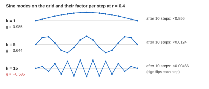
Short waves have large k and shrink much faster. At r = 0.4 mode 1 keeps 0.985 of itself per step, mode 5 only 0.644. Starting from 50·sin(πx/16) + 30·sin(5πx/16), after 10 steps the coefficients are 42.8 and 0.37: the wiggle is gone and one hump remains. That is why diffusion smooths. It also explains the blow-up: the shortest wave, k = 15, has the factor that leaves [−1, 1] first, at r > 1/2. (Demo: high frequencies die first)

Sine modes k = 1, 5 and 15 sampled on 17 grid points with their factors per step at r = 0.4: 0.985, 0.644 and −0.585; after 10 steps they keep 0.856, 0.0124 and 0.00466 of their size — The faster a mode wiggles, the smaller its factor per step, so short waves vanish first.

Other ways to step an equation in time are on Runge–Kutta vs Euler; a single mode decaying like e^−γt is the same exponential as in damped oscillation.

What the page leaves out

Only the explicit scheme on a short 1-D rod is shown. Implicit schemes (backward Euler, Crank–Nicolson) solve a tridiagonal system each step and are stable for any r, so real solvers can take large time steps. Real rods also have ends at other temperatures, heat sources, materials whose α varies along the rod, and two or three dimensions, where the limit becomes r ≤ 1/4 or 1/6. The exact solution of the continuous equation, a Gaussian spreading like √(4αt), is only hinted at by the spike.