The idea: f(x) gets as close to L as you like when x is close enough to a
A limit describes what f does near a point a, not at it. We write limx→a f(x) = L when the values f(x) can be kept as close to L as anyone asks, just by taking x close enough to a. The value f(a) itself plays no part: it may be different, or missing.
The ε–δ definition
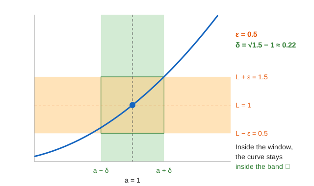
"As close as you like" is made exact with two numbers. Someone picks a tolerance ε > 0: the orange band from L − ε to L + ε. You must answer with a δ > 0: the green window from a − δ to a + δ, such that
0 < |x − a| < δ ⟹ |f(x) − L| < ε
If you can answer every ε, the limit is L. The "0 <" leaves out x = a itself. Each Shrink ε halves the band and the page draws the widest window that still works. For f(x) = x² at a = 1 the right side is the tighter one, so δ = √(1 + ε) − 1:
| ε | δ = √(1 + ε) − 1 | δ / ε |
|---|---|---|
| 1 | 0.414 | 0.41 |
| 0.5 | 0.225 | 0.45 |
| 0.25 | 0.118 | 0.47 |
| 0.125 | 0.0607 | 0.49 |
| 0.0625 | 0.0308 | 0.49 |
A smaller ε forces a smaller δ. Here δ is about ε / 2 because the slope of x² at 1 is 2: a steep curve needs a narrow window. (Demo: ε–δ for x² at a = 1)
One-sided limits and the table
Approach a sets x = a − h (from the left) and x = a + h (from the right) for h = 0.5, 0.1, 0.01, 0.001, 0.0001, and writes f in two columns. If the left column settles on a number, that is the left limit limx→a⁻ f(x); the right column gives the right limit limx→a⁺ f(x). The limit exists exactly when both exist and are equal.
| h | x² at 1−h | x² at 1+h | step at 1−h | step at 1+h |
|---|---|---|---|---|
| 0.5 | 0.25 | 2.25 | 0.5 | 2.5 |
| 0.1 | 0.81 | 1.21 | 0.9 | 2.1 |
| 0.01 | 0.9801 | 1.0201 | 0.99 | 2.01 |
| → | 1 | 1 | 1 | 2 |
A table is evidence, not proof: it only samples a few x. sin(1/x) shows why. Its table looks random, and a cleverer choice of h could even make it look constant (h = 1/(2πk) gives 0 every time).
Four ways a limit fails (or f(a) spoils it)
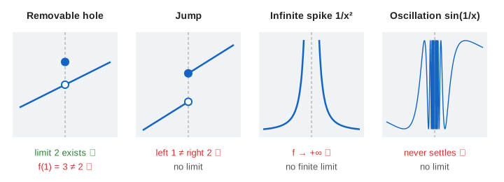
- Removable hole. (x² − 1)/(x − 1) is x + 1 for every x ≠ 1, so both sides go to 2. The extra point f(1) = 3 sits above the hole and the ε–δ window ignores it. (Demo: removable hole)
- Jump. x for x < 1 and x + 1 for x ≥ 1: left limit 1, right limit 2. With L = 1.5, ε = 1 still works (δ = 0.5), but ε = 0.5 fails for every δ: no band thinner than the jump can hold both sides. (Demo: jump)
- Infinite spike. 1/x² gives 4, 100, 10⁴, 10⁶, 10⁸ as h shrinks. We write lim = +∞, but that means "no finite limit": every band around any L is left behind. (Demo: infinite spike) The line x = 0 is then a vertical asymptote; see Types of Asymptotes.
- Oscillation. sin(1/x) hits 1 at x = 1/(π/2 + 2πk) and −1 halfway between, for every k. Every window around 0 holds both, so no L is within ε < 1 of all the values. (Demo: oscillation)
Continuity: three conditions
f is continuous at a when limx→a f(x) = f(a). Spelled out, that is three checks, and Continuous? runs them in order:
- f(a) is defined;
- limx→a f(x) exists (left = right, finite);
- the two are equal.
| f at a | 1. f(a) | 2. limit | 3. equal | verdict |
|---|---|---|---|---|
| x² at 1 | 1 ✓ | 1 ✓ | ✓ | continuous |
| hole at 1 | 3 ✓ | 2 ✓ | ✗ | removable: set f(1) = 2 |
| step at 1 | 2 ✓ | 1 ≠ 2 ✗ | ✗ | jump |
| 1/x² at 0 | none ✗ | +∞ ✗ | ✗ | infinite |
| sin(1/x) at 0 | none ✗ | none ✗ | ✗ | oscillating |
Only the removable kind can be repaired by changing one value. Polynomials, eˣ, sin and cos are continuous everywhere, and sums, products and compositions of continuous functions are continuous, so most limits are found by just plugging in a. That is what makes the hole interesting: plugging in gives 0/0, and the limit has to be found another way (here, by cancelling x − 1).
Where limits come next
- The derivative is a limit of slopes: Derivative as a Limit, and zooming in until a curve looks straight in Local Linearity. A function must be continuous at a to have a derivative there.
- The integral is a limit of sums: Riemann Sums and the Fundamental Theorem. The spike 1/x² comes back in Improper Integrals, where an area can stay finite near an infinite spike.
- Continuity on an interval is what the Mean Value Theorem needs, and what lets Newton's method and bisection trap a root between a sign change.
Continuity is what makes bisection work: a continuous f that changes sign must cross zero, see Root Finding: Bisection vs Newton vs Secant.
What the page leaves out
The page computes δ from exact formulas for these five functions instead of proving it in general. Limits at infinity (x → ∞), the limit laws, the squeeze theorem (which proves sin x / x → 1 and x·sin(1/x) → 0), L'Hôpital's rule, uniform continuity, and limits of functions of several variables are not covered. The table uses double-precision arithmetic, so the hole's values carry rounding in the last digits.