MariaDB Histograms Visualization | Where Row Estimates Come From

The idea: a cost is only as good as its row estimate

A cost-based optimizer estimates the cost of each way to run a query and keeps the cheapest. The book lists five cost components: disk access, temporary storage, CPU, memory and communication. MariaDB's cost model counts mainly the first and the third: pages read from storage and rows processed by the CPU. Both depend on one number: how many rows each step returns. That number comes from the selectivity of each condition, the share of rows that pass it.

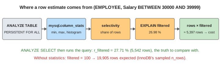
Pipeline: ANALYZE TABLE fills the mysql statistics tables; the optimizer turns them into a selectivity, EXPLAIN shows it as filtered, and rows times filtered gives the estimated row count used for costs. — Statistics → selectivity → filtered → estimated rows → cost. A wrong histogram makes every later number wrong.

The page uses one table and one condition type. EMPLOYEE has 20,000 rows and a skewed Salary between 30,000 and 499,929, the range of the book's Figure 19.4. There is no index on Salary, so the plan is always a full scan (type = ALL). Only the estimate changes. Every statistic, histogram and percentage on the canvas was produced by MariaDB 13.1 on this table.

The catalog in MariaDB

The book says the optimizer reads the size of each file and the distribution of values from the catalog. MariaDB keeps two sets. InnoDB keeps sampled numbers by itself (mysql.innodb_table_stats.n_rows = 19,905 here, not quite 20,000). The engine-independent statistics are exact, and you collect them yourself:

Book	MariaDB	EMPLOYEE
r, number of records	`mysql.table_stats.cardinality`	20000
NDV(A, R), distinct values	r / `column_stats.avg_frequency`	Salary: 20000 / 1.0862 ≈ 18,412
s = sl · r, rows per value	`column_stats.avg_frequency`	Dno: 400
value range	`column_stats.min_value`, `max_value`	30000 … 499929
(not in the book)	`column_stats.nulls_ratio`, `avg_length`	0.0000, 4.0000
histogram	`column_stats.hist_type`, `histogram`	see below
rows per index key	`mysql.index_stats.avg_frequency` per prefix	idx_dno: 400

They are filled by ANALYZE TABLE EMPLOYEE PERSISTENT FOR ALL (or FOR COLUMNS (…) INDEXES (…)). With the default use_stat_tables = PREFERABLY_FOR_QUERIES, a plain ANALYZE TABLE only refreshes InnoDB's numbers, and the optimizer uses the mysql tables whenever they have a row. MariaDB keeps no histogram for Ssn: it is the only column of the primary key.

Without a histogram: the uniform guess

With no column statistics at all, MariaDB cannot estimate a condition on an unindexed column. EXPLAIN shows filtered = 100 (Demo 1). With only min and max (histogram_size = 0) it makes the book's assumption that values are spread evenly:

sel = \frac{hi - lo}{\max - \min} = \frac{39999 - 30000}{499929 - 30000} = 2.13 %

The real share is 27.71 %, so the estimate is 13× too low. For Salary >= 200000 it is 63.82 % against 28.75 %, more than 2× too high (Demo 2). An equality uses avg_frequency / cardinality: about 1 row for Salary = 30000, which really has 258.

Height-balanced histograms: DOUBLE_PREC_HB and JSON_HB

The book describes equi-width buckets (equal value ranges) and equi-height buckets (equal numbers of rows), and calls equi-height better. MariaDB only builds equi-height ones, which it calls height-balanced. The type is set by histogram_type and the size by histogram_size (default 254):

	`DOUBLE_PREC_HB`	`JSON_HB`
default	MariaDB 10.4 to 10.11	MariaDB 11.0 and later (exists since 10.8)
what `histogram_size` means	bytes: 2 per endpoint, so 20 → 10 endpoints → 11 buckets	number of buckets
a bucket stores	its end as a 16-bit position between min and max	exact start value, `size` (share of rows), `ndv`
a range	counts every bucket it touches, 1/(n+1) each	full buckets + an even share of the edge buckets
a frequent value	can span several buckets	gets a bucket of its own with `ndv = 1`

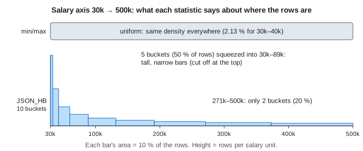
On a salary axis from 30k to 500k, the uniform guess is one flat block, while the 10 JSON_HB buckets each hold 10 percent of the rows: five of them are squeezed into 30k to 89k and the last two cover 271k to 500k. — Every JSON_HB bucket holds 10 % of the rows, so crowded low salaries get narrow buckets, the opposite of the uniform guess.

With 10 JSON_HB buckets, Salary BETWEEN 30000 AND 39999 covers buckets 0 and 1 fully (20.0 %) and 69.7 % of bucket 2, 33765–42709 (7.0 %): 26.98 % against the real 27.71 % (Demo 3). DOUBLE_PREC_HB with 11 buckets touches four of them and says 4/11 = 36.36 % (Demo 4). With the default 254 the estimates are almost exact:

WHERE	min/max	DOUBLE_PREC_HB 20	DOUBLE_PREC_HB 254	JSON_HB 10	JSON_HB 254	real
30000–39999	2.13	36.36	28.13	26.98	27.71	27.71
40000–69999	6.38	18.18	17.19	16.48	16.28	16.28
70000–119999	10.64	27.27	14.06	13.84	13.65	13.65
120000–199999	17.02	18.18	14.84	13.81	13.61	13.61
>= 200000	63.82	27.27	28.13	28.89	28.75	28.75
= 30000	0.01	0.01	2.34	0.02	1.29	1.29

The last row is the book's point about granularity. 258 rows have Salary = 30000. In a 10-bucket histogram they hide inside a bucket of 471 values, so JSON_HB guesses size / ndv = 0.02 %. With 254 buckets, 30000 fills a bucket by itself and the estimate is exact (Demo 5).

optimizer_use_condition_selectivity

Statistics in the tables are not enough: this variable decides which conditions get a selectivity at all.

Value	Uses	Salary 30000–39999
1	only conditions on indexed columns (the MariaDB 5.5 behaviour)	100
2	range conditions an index can check	100
3	all range conditions, from min/max	2.13
4 (default since 10.4)	all range conditions, with histograms	26.98
5	like 4, plus sampling for some non-range conditions	26.98

Demo 6 switches between 1, 3 and 4 with the same 10-bucket histogram in place.

Reading filtered and r_filtered

EXPLAIN EXTENDED, EXPLAIN FORMAT=JSON and ANALYZE show filtered: the estimated percentage of the rows examined that pass the table's conditions. rows × filtered is what the optimizer expects the next step to receive, and in a join it multiplies into the cost of every later table. ANALYZE SELECT also runs the query and adds r_rows and r_filtered, the measured values. When filtered and r_filtered differ by several times, collect statistics or add a histogram. The canvas shows tabular ANALYZE output, without its possible_keys, key_len and ref columns (all NULL here).

See also How a Query Planner Picks a Plan (PostgreSQL) for the same idea with pg_stats, and MySQL Index Access Paths and EXPLAIN for what changes when the column has an index.

What the page leaves out

The book's compiled vs interpreted queries (MariaDB optimizes every statement when it runs and has no stored plans), and catalog numbers MariaDB does not keep: block counts b, blocking factor bfr and index levels x come from the storage engine, not from a catalog table. Also left out: equi-width histograms (MariaDB has none), the older SINGLE_PREC_HB type, sampling with analyze_sample_percentage, histograms on several columns together (MariaDB has none, so correlated conditions are multiplied as if independent), the selectivity of conditions on indexed columns, which comes from the index (range estimates by index dives), and how filtered feeds join order and costs.

See where this page fits on the Databases & Storage mind map.