MariaDB Cost-Based Optimization: a Worked Example

The idea: price every plan from the catalog

A cost-based optimizer never looks at the data while it plans. It reads a few numbers from the catalog (rows, blocks, distinct values, index levels), estimates the cost of each candidate plan from them, and runs the cheapest one. This page follows the textbook example of Elmasri & Navathe (section 19.6) for query Q2, then shows what MariaDB does with the same query on data that matches the book's statistics.

Q2: SELECT Pnumber, Dnum, Lname, Address, Bdate
    FROM   PROJECT, DEPARTMENT, EMPLOYEE
    WHERE  Dnum = Dnumber AND Mgr_ssn = Ssn AND Plocation = 'Stafford';

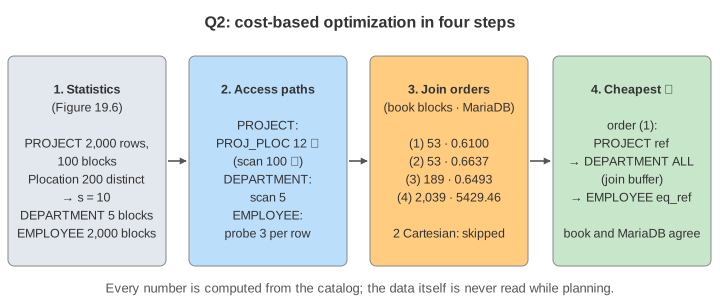
The statistics of Figure 19.6

Table	Rows	Blocks	Index
PROJECT	2,000	100	PROJ_PLOC on Plocation, nonunique, 200 distinct keys, Blevel 1
DEPARTMENT	50	5	none
EMPLOYEE	10,000	2,000	EMP_SSN on Ssn, unique, Blevel 1

Blevel counts the levels above the leaves, so both indexes have x = 2 levels (root + leaf). With 200 distinct locations and a uniform spread, the selectivity of Plocation = 'Stafford' is 1/200, so s = 2,000 / 200 = 10 projects. MariaDB keeps the same kind of numbers: ANALYZE TABLE … PERSISTENT FOR ALL fills mysql.column_stats, where it stores avg_frequency (rows per distinct value: 10.0 for Plocation) instead of the number of distinct values.

Access paths for each table

• PROJECT: a table scan reads 100 blocks; PROJ_PLOC costs x + s = 2 + 10 = 12. The index wins. MariaDB shows type ref, key PROJ_PLOC, ref const, and its optimizer trace lists the scan with "chosen": false, "cause": "cost".
• DEPARTMENT: no index, so a 5-block scan is the only path. MariaDB: type ALL.
• EMPLOYEE: when it comes after DEPARTMENT, each Mgr_ssn is one probe of EMP_SSN, x + 1 = 3 blocks. In MariaDB, Ssn is the PRIMARY KEY (InnoDB's clustered index), so the probe is type eq_ref on PRIMARY.

Demo: access paths for each table.

Four left-deep join orders

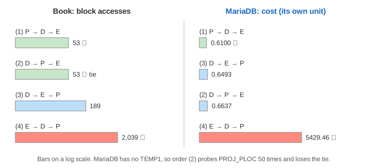
Like the book, MariaDB only builds left-deep plans: each join adds one base table to the result so far. Three tables give 3! = 6 orders, but PROJECT and EMPLOYEE share no join condition, so the two orders that join them first are Cartesian products and are not costed. That leaves:

Order	Book block accesses	MariaDB cost
(1) PROJECT → DEPARTMENT → EMPLOYEE	12 + 1 + 6 + 2 + 32 = 53	0.6100 ✓ cheapest
(2) DEPARTMENT → PROJECT → EMPLOYEE	53 (a tie)	0.6637
(3) DEPARTMENT → EMPLOYEE → PROJECT	189	0.6493
(4) EMPLOYEE → DEPARTMENT → PROJECT	2,039	5429.46

The book works out order (1) only and leaves the others "as an exercise". Orders (2) to (4) here use exactly the same rules: the selection on PROJECT is done first into TEMP1 (12 + 1 block write), every join result is written to a temporary file (5 rows per block), joins are nested loops, and a small input stays in the buffer so it is read once. MariaDB's costs come from EXPLAIN FORMAT=JSON with each order forced by SELECT STRAIGHT_JOIN, which joins the tables in FROM-clause order.

Costing order (1) step by step

1. Select the Stafford projects through PROJ_PLOC: 12. Write them to TEMP1: 10 rows at 20 rows per block = 1 block.
2. Join TEMP1 with DEPARTMENT. TEMP1 fits in the buffer, so DEPARTMENT's 5 blocks are read once: 1 + 5 = 6. Dnumber is DEPARTMENT's key, so TEMP2 has 10 rows = 2 blocks.
3. Join TEMP2 with EMPLOYEE through EMP_SSN: 2 + 10 × 3 = 32.
4. The projection is pipelined: 0. Total 12 + 1 + 6 + 2 + 32 = 53 (52 if the TEMP1 write is not counted; the book only lists the parts).

Order (1) is cheap because it starts from the most selective piece: every later step works on 10 rows. Order (3) does 50 manager lookups before the Stafford filter, and order (4) scans all 2,000 EMPLOYEE blocks. Demo: order (1), the book's worked example; Demo: order (4), the full EMPLOYEE scan.

What MariaDB picks, and where it differs

For Q2 as written, MariaDB's optimizer picks order (1), the same as the book:

id	table	type	key	ref	rows	filtered	Extra
1	PROJECT	ref	PROJ_PLOC	const	10	100.00	Using index condition
1	DEPARTMENT	ALL	NULL	NULL	50	100.00	Using where; Using join buffer (flat, BNL join)
1	EMPLOYEE	eq_ref	PRIMARY	company.DEPARTMENT.Mgr_ssn	1	100.00

• No temporary files. The book materializes TEMP1 and TEMP2. MariaDB pipelines rows through nested loops; the 10 projects wait in a join buffer (Using join buffer (flat, BNL join)), so DEPARTMENT is scanned once, which is the book's "TEMP1 fits in the buffer".
• No tie. Without TEMP1, order (2) probes PROJ_PLOC once per department, 50 times, so it costs more than order (1). Demo: order (2), a tie in the book.
• A cruder row estimate. The book knows Dnumber is DEPARTMENT's key, so 10 rows come out of the first join. DEPARTMENT has no index, so MariaDB does not know that: it guesses 10 × 50 = 500 rows (filtered 100.00). ANALYZE shows the truth, r_filtered 2.00 on DEPARTMENT.
• Different units. MariaDB's cost is its own number, mixing I/O and CPU per row, not a count of blocks. Compare rankings, not values.

Demo: MariaDB's choice. How MariaDB searches the orders (greedy search, optimizer_search_depth, optimizer_prune_level) is shown in MariaDB: How the Optimizer Picks a Join Order. See also How a Query Planner Picks a Plan for the same ideas in PostgreSQL, Nested Loop vs Hash Join vs Merge Join and MySQL Index Access Paths and EXPLAIN.

What the page leaves out

The book's other join methods (sort-merge join) and its materialized TEMP files, which MariaDB does not use for this query; MariaDB's hash join variants (join_cache_level), histograms and optimizer_use_condition_selectivity, which would sharpen the 500-row guess; how the optimizer searches and prunes the orders; and real timings, which vary between runs (on a test machine order (1) took 0.03 ms and order (4) 25 ms).

References

EXPLAIN (MariaDB Knowledge Base)

Optimizer Trace Overview (MariaDB Knowledge Base)

Engine-Independent Table Statistics (MariaDB Knowledge Base)

Block-Based Join Algorithms (MariaDB Knowledge Base)