The idea: one dataset, two opposite answers
A 1986 study compared two treatments for kidney stones: A, open surgery, and B, a keyhole method (percutaneous nephrolithotomy, PCNL). Put all 700 patients together and B looks better: 83% recovered against 78%. Split the same patients by the size of their stone and A is better for small stones and better for large stones. A trend that holds in every group and reverses when the groups are combined is Simpson's paradox.
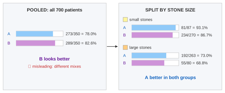
The page draws both views side by side on the same counts. Pool fills the left panel, Split the right one, Show Mix explains the flip, and Randomize shows the fix (Demo 1: kidney stones, pooled vs split).
The kidney-stone numbers
| Small stones | Large stones | All | |
|---|---|---|---|
| A: open surgery | 81 / 87 = 93.1% | 192 / 263 = 73.0% | 273 / 350 = 78.0% |
| B: keyhole (PCNL) | 234 / 270 = 86.7% | 55 / 80 = 68.8% | 289 / 350 = 82.6% |
Nothing is miscounted: 81 + 192 = 273 and 87 + 263 = 350. The only thing that changed between the two views is how the patients are grouped.
Confounders
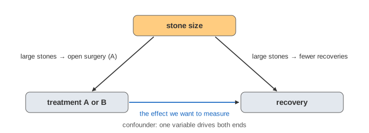
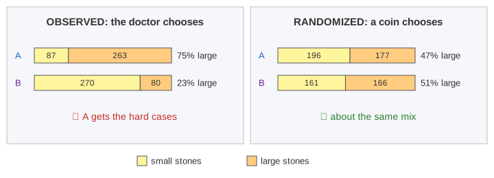
Look at who got which treatment. 263 of A's 350 patients (75%) had large stones; only 80 of B's 350 (23%) did. Large stones are harder to treat with anything, and doctors chose the stronger treatment, open surgery, for the hard cases. Stone size affects both which treatment a patient gets and whether the patient recovers. A variable like that is a confounder: it creates a link between treatment and outcome that is not caused by the treatment.
Overall rates are weighted averages
An arm's overall rate is the average of its group rates, weighted by how many of its patients are in each group:
A's average leans on its large-stone rate, B's on its small-stone rate. The plot at the bottom right draws this: each arm is a line from its small-stone rate (left) to its large-stone rate (right), and its overall rate is the point on the line at its own share of large stones. A's line is above B's everywhere, but A's dot sits far to the right and B's far to the left, so B's dot ends up higher (Demo 2: why it flips). This chart is sometimes called a Baker–Kramer plot.
Correlation is not causation
The pooled table shows a correlation: patients who got B recovered more often. It does not show that B causes more recoveries. A correlation can come from the cause you are looking at, from a confounder that drives both variables, from chance, or from the way the data was selected. Ice-cream sales and drownings rise together because of summer, not because one causes the other. The same reasoning applies to a fitted regression line: a slope says how the variables move together in this data, not what would happen if you changed one of them.
Why randomized experiments fix it
In a randomized controlled trial a coin, not the doctor, decides who gets which treatment. The coin knows nothing about the stones, so both arms get about the same mix of small and large stones, and of every other trait, measured or not. Then the only systematic difference between the arms is the treatment. On the page, Randomize gives each of the same 700 patients A or B by a seeded coin flip: A gets 196 small + 177 large, B gets 161 + 166 (47% and 51% large). With each group recovering at the rate it had in the study, A wins pooled, 311 / 373 = 83.4% against 254 / 327 = 77.7%, and in both groups: no flip (Demo 3: randomize the treatment).
This is why online A/B tests hash users into variants at random instead of comparing users who chose a feature with users who didn't.
Admissions: the same pattern
A famous case is the 1973 graduate admissions at UC Berkeley: men were admitted more often overall, but in most departments women were admitted at the same or a higher rate. Women had applied more often to departments that rejected most applicants. The admissions data on the page uses simplified, illustrative numbers for two departments:
| Dept X (easy) | Dept Y (hard) | All | |
|---|---|---|---|
| A: women | 70 / 100 = 70% | 135 / 900 = 15% | 205 / 1000 = 20.5% |
| B: men | 480 / 800 = 60% | 20 / 200 = 10% | 500 / 1000 = 50% |
Here the confounder is the department, and you can't randomize anyone's sex. The fix is to stratify: compare within each department, as the split panel does (Demo 4: admissions).
Which answer is right?
The numbers alone can't say whether to trust the pooled or the split view. You need to know how the data came about. If the grouping variable is a cause of both treatment and outcome (stone size, department), split on it. If it is a result of the treatment, for example blood pressure measured after a drug was given, splitting on it hides part of the drug's effect, and the pooled view is the right one. Causal diagrams make that choice explicit; conditional probability is the arithmetic underneath both views.
What the page leaves out
Sampling noise and confidence intervals (the counts are taken as exact), more than two strata or several confounders at once, regression adjustment, propensity scores and matching, Pearl's back-door criterion and do-calculus for choosing what to adjust for, the full six-department Berkeley data, and continuous versions of the paradox where a regression slope reverses inside each group.