The idea: reuse what a big model already learned
Training a good image model needs a lot of photos. Transfer learning skips most of that work. Take a network that was already trained on a big dataset, keep the part that turns a photo into useful features (the backbone), and replace only the last layer that picks the class (the head). Then train on your own, much smaller dataset.
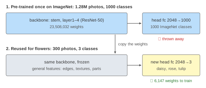
The page uses ResNet-50 trained on ImageNet (1.28 million photos, 1000 classes). The new task is to tell three flowers apart: daisy, rose and tulip. The parameter counts are the real ones from torchvision. The accuracy numbers are illustrative: they have the usual shape of such runs, but they are not from a live training run in your browser.
What the layers learn
A CNN builds its features in layers (see Convolution in a CNN). The first layers find edges and colours. The middle layers combine them into textures and parts such as petals, eyes or wheels. The last block, layer4, finds whole object shapes that fit the 1000 ImageNet classes. Early features are useful for almost any photo. Late features are more specific to the old task. Yosinski et al. (2014) measured this: features get less transferable the higher the layer.
Three ways to train
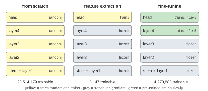
- From scratch: every weight starts random and all 23,514,179 weights learn from your photos alone (Demo 2).
- Feature extraction: keep the ImageNet weights, freeze the whole backbone (
requires_grad = Falsein PyTorch,trainable = Falsein Keras) and train only the new head: 6,147 weights. The gradient stops at the head, so each step is cheap (Demo 1). - Fine-tuning: start from the feature-extraction result, unfreeze the top block (layer4) and keep training it with the head at a small learning rate (Demo 3).
| 300 photos, 10 epochs | trainable weights | train | validation |
|---|---|---|---|
| from scratch | 23,514,179 | 98% | 53% ✗ |
| feature extraction | 6,147 | 89% | 84% |
| fine-tune layer4, lr 1e-5 | 14,970,883 | 97% | 90% ✓ |
| fine-tune layer4, lr 1e-2 | 14,970,883 | 99% | 62% ✗ |
From scratch, 300 photos are far too few for 23.5 million weights. The network memorises the training photos: train accuracy reaches 98%, but validation peaks at 56% and then falls to 53%. That gap is overfitting. Feature extraction reaches 84% because the frozen ImageNet features already separate the flowers well; the head only has to draw the lines between them.
Head first, then a small learning rate
Fine-tuning has an order. A new head starts random. If layer4 were unfrozen right away, the large, random gradients from that head would flow into layer4 and spoil its pre-trained weights. So the head is trained first with the backbone frozen; only then is layer4 unfrozen. On the page, choosing a fine-tune strategy runs feature extraction first if it has not been done.
The learning rate for fine-tuning is small, here 1e-5, a hundred times smaller than the 1e-3 used for the head. The pre-trained weights are already good, so they should only move a little. Validation goes from 84% to 90% (Demo 3). With lr 1e-2 the steps are so large that layer4 forgets what it learned on ImageNet, and with 300 photos there is not enough data to learn it back. Validation drops to 62% while train accuracy climbs to 99% (Demo 4). Forgetting old knowledge this way is called catastrophic forgetting.
Fine-tuning also has a trap with batch normalization: its layers keep running statistics from ImageNet. Keras recommends keeping them in inference mode while fine-tuning a small dataset (see Dropout & Batch Normalization).
When to use which
With 30,000 photos, training from scratch reaches 84%, close to feature extraction at 88%, and fine-tuning still wins with 94% (Demo 6). Two questions decide the choice: how much data you have, and how similar it is to the data the model was trained on.
| similar to ImageNet | very different (X-rays, satellite images) | |
|---|---|---|
| little data | feature extraction | feature extraction from an earlier layer, or fine-tune with care |
| a lot of data | fine-tune the top blocks | fine-tune more blocks, or train from scratch |
The same idea runs through modern AI. Language models are pre-trained once on a huge text corpus and then fine-tuned for a task. LoRA makes that fine-tuning cheaper by freezing the big weight matrices and training small low-rank ones next to them. Knowledge distillation moves knowledge the other way: from a big trained model into a smaller one. CNN vs Transformer compares the two kinds of backbone you would download.
See also Object Detection: IoU, Non-Maximum Suppression and AP for the last step of a detector built on a pre-trained backbone.
See also A CNN Layer by Layer for counting the parameters of each layer, and why a global average pooling head is so small.
What the page leaves out
A real training run (the curves are illustrative); data augmentation; caching the frozen features once so feature extraction runs even faster; discriminative learning rates (a different lr per block) and gradual unfreezing (ULMFiT); fine-tuning every block; domain adaptation when the new data comes from a different distribution; and self-supervised pre-training (SimCLR, DINO) instead of ImageNet labels.