The idea: one long table of numbers, a few small tables of words
A shop's order system keeps its data in many small normalized tables, so that every fact is stored once and an order is quick to write. A report asks a different kind of question: how much did we sell, by category, by quarter, by country? A data warehouse reshapes the same data for that question. The numbers go into one long fact table, one row per order line. The words you group and filter by go into a few small dimension tables. Drawn with the fact table in the middle, the picture is a star schema. The page stores 144 order lines in such a star and shows the answers as a grid, the OLAP cube view.
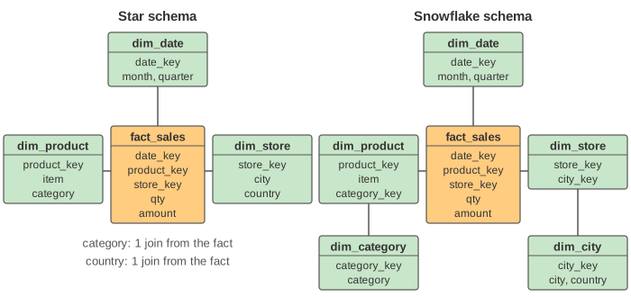
From the order tables to a star
The normalized model has six tables: orders, order_items, products, categories, stores, cities. The warehouse load turns them into four (Demo: normalized orders → star schema):
orders+order_itemsbecomefact_sales: keys to the dimensions plus the measuresqtyandamount. The amount isqty × price, worked out once at load time.- The order date becomes a key into
dim_date, which has the month, quarter and year written out for every day. products+categoriesbecomedim_product, andstores+citiesbecomedim_store. The category and country text now repeats in many rows. That breaks third normal form on purpose: dimensions are small, and nobody updates them row by row.
For the start view (category by quarter) the normalized tables need 3 joins and two computed expressions, QUARTER(o.order_date) and oi.qty * oi.price. The star needs 2 joins and reads stored columns. The grid shows the same numbers in both. A view only joins the dimensions it uses: the coloured boxes on the canvas are the tables in the current query.
Star or snowflake
A snowflake schema normalizes the dimensions again: dim_product keeps a category_key and the name moves to dim_category; city and country move to dim_city. With the view sliced to Vietnam, the star's query has 3 joins and the snowflake's has 5, for the same 72 fact rows and the same total, 509 (Demo: star vs snowflake).
| Star | Snowflake | |
|---|---|---|
| Dimension tables | one wide table per dimension | a chain of tables per dimension |
| Repeated text | yes (category in every product row) | no |
| Joins to reach a category or country | 1 | 2 |
| Queries | shorter, fewer joins | longer |
| Space saved by splitting | — | little: dimensions are tiny next to the fact table |
That is why most warehouses choose the star. See also Database Normalization: 1NF, 2NF and 3NF for how the order tables got their shape, and ER Model to Tables for keys and foreign keys.
The cube and its hierarchies
Each dimension is one axis of a cube: Time × Product × Store. A cell of the cube holds the sum of the measure for one combination, for example Laptop, Jan, Tokyo. Each dimension also has a concept hierarchy, a ladder from fine to coarse: month → quarter → all, item → category → all, city → country → all. A view of the cube picks one level per dimension. In SQL the picked levels are the GROUP BY columns, and a dimension at "all" is simply not in the GROUP BY.
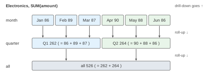
Roll-up and drill-down
Roll-up climbs one level of one hierarchy: months are added into quarters, and 18 groups become 6. Drill-down goes the other way: Laptop Q1 = 148 opens into Jan 49, Feb 51 and Mar 48 (Demo: roll up month → quarter → all, Demo: drill down to item × month). Both read the same fact rows and keep the same grand total, 1098. Only one column of the GROUP BY changes:
SELECT p.category, d.month, SUM(f.amount)        -- 18 groups
FROM fact_sales f
  JOIN dim_product p USING (product_key)
  JOIN dim_date d USING (date_key)
GROUP BY p.category, d.month;

... GROUP BY p.category, d.quarter;              -- roll up: 6 groups
... GROUP BY p.category;                         -- roll up again: 3 groups, dim_date not joined
MariaDB can add the rolled-up rows to one result: GROUP BY p.category, d.quarter WITH ROLLUP returns the 6 groups, a subtotal row per category and a grand total row. See also How a SELECT Runs: WHERE, GROUP BY, HAVING, ORDER BY for what the server does with these clauses.
Slice, dice and pivot
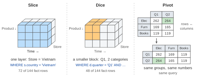
A slice fixes one dimension to one value. With WHERE s.country = 'Vietnam' the query reads 72 of the 144 fact rows, and Electronics Q1 drops from 262 to 125 (Demo: slice Store = Vietnam, then Tokyo). A dice picks values on two or more dimensions: WHERE d.quarter = 'Q1' AND p.category IN ('Electronics', 'Furniture') keeps 48 fact rows (Demo: dice Q1 × two categories). Both are a WHERE. They change which rows are summed, not how the rows are grouped.
A pivot swaps the rows and the columns of the grid (Demo: pivot rows and columns). The groups and the numbers stay the same, and so does the query: SQL returns one row per group, and laying those rows out as a grid is the job of the reporting tool. To get a grid straight from MariaDB, write one conditional sum per column: SUM(CASE WHEN d.quarter = 'Q1' THEN f.amount END) AS Q1.
| Operation | What changes in the query | Fact rows read | Groups |
|---|---|---|---|
| Roll-up | a GROUP BY column goes one level up, or leaves | same | fewer |
| Drill-down | a GROUP BY column goes one level down, or is added | same | more |
| Slice | one WHERE condition on one dimension | fewer | same levels |
| Dice | WHERE conditions on two or more dimensions | fewer | fewer |
| Pivot | nothing (column order only) | same | same |
See also Row store vs Column store for why warehouses store the fact table by column, and MariaDB Table Elimination for the optimizer dropping a join the query does not need.
See also ETL and Slowly Changing Dimensions for how the fact and dimension tables get loaded, and what happens to a report when a dimension row changes.
See also Pandas GroupBy, which shows grouping by one and by two keys in pandas, the building block of a roll-up.
What the page leaves out
A real fact table has millions of rows and is sparse: most combinations of day, product and store have no sale. Here every one of the 144 combinations has exactly one row, there is one year, and the date dimension stops at the month. The page leaves out how the warehouse is loaded (ETL), slowly changing dimensions, more than one measure, and measures that cannot be added up (an average or a distinct count cannot be rolled up from the level below). OLAP servers store precomputed aggregates to answer roll-ups without reading the fact table; MariaDB has no materialized views, so there a summary table has to be filled by hand. MariaDB has WITH ROLLUP but not GROUP BY CUBE or GROUPING SETS, and no PIVOT keyword. The pivot here only swaps the two axes on the grid; a full rotate could also bring Store onto an axis.