The idea: tables in, table out
Relational algebra is a small set of operators on tables (relations). Each operator takes one or two tables and returns a new table. Because the output is a table again, operators can be nested: a query is a tree of operators with the stored tables at the leaves. SQL says what you want; the database turns it into such a tree and runs it. Every plan you see in EXPLAIN is made of these operators, or of faster ways to compute them.
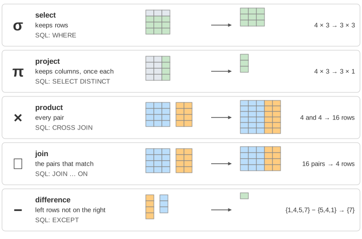
The data on the canvas
Two tables cut down from the COMPANY database of Elmasri & Navathe: EMPLOYEE(Fname, Salary, Dno) with Smith, Wong, Wallace and Borg, and DEPARTMENT(Dnumber, Dname) with Headquarters, Administration and Research. Sales (7) was added and has no employee, so the join and the difference have something to show. Every answer can be checked by hand.
σ select and π project
σ (select) keeps the rows that pass a condition and keeps all the columns. σ Salary>35000 (EMPLOYEE) tests 4 rows and returns Wong, Wallace and Borg. In SQL it is the WHERE clause; the SQL keyword SELECT is not σ (Demo: σ keeps the rows that pass).
π (project) keeps the listed columns and drops the others. A relation is a set, so the result holds each row once: π Dno (EMPLOYEE) is {5, 4, 1}, not 5, 5, 4, 1. SQL tables are bags (multisets) and keep the duplicate unless you write DISTINCT (Demo: π keeps columns, drops duplicates).
× product and ⋈ join
× (Cartesian product) glues every row of one table to every row of the other: 4 × 4 = 16 rows with 3 + 2 = 5 columns. Most of them are nonsense (Smith paired with Sales), which is why it is rarely used alone (Demo: × pairs every row with every row).
⋈ (join) is a product followed by a selection: EMPLOYEE ⋈ Dno=Dnumber DEPARTMENT = σ Dno=Dnumber (EMPLOYEE × DEPARTMENT). The canvas compares all 16 pairs and keeps 4. A join with any condition is a theta join; with only = it is an equijoin; a natural join (*) joins on the columns with the same name and keeps one copy of them. A row with no partner, like Sales, is not in the result; the outer joins (⟕ LEFT, ⟖ RIGHT, ⟗ FULL) keep it and fill the other side with NULL (Demo: ⋈ is σ over ×, Sales drops out).
Set operators: ∪, −, ∩
∪ union, − difference and ∩ intersection work on two tables that are union compatible: the same number of columns, with matching types. EMPLOYEE and DEPARTMENT are not, so the page first projects each to one number column. π Dnumber (DEPARTMENT) − π Dno (EMPLOYEE) = {1, 4, 5, 7} − {5, 4, 1} = {7}: the departments with no employee (Demo: − finds the department with no one). Difference is how relational algebra says "no" or "not exists".
| Operator | Symbol | SQL (MariaDB) | Rows of the result |
|---|---|---|---|
| select | σc(R) | WHERE c | ≤ |R| |
| project | πcols(R) | SELECT DISTINCT cols | ≤ |R| |
| product | R × S | CROSS JOIN, or FROM R, S | |R| · |S| |
| join | R ⋈c S | JOIN … ON c | 0 to |R| · |S| |
| union | R ∪ S | UNION | ≤ |R| + |S| |
| difference | R − S | EXCEPT, NOT EXISTS | ≤ |R| |
| intersection | R ∩ S | INTERSECT | ≤ min(|R|, |S|) |
| rename | ρT(R) | AS T | |R| |
MariaDB has EXCEPT and INTERSECT since 10.3, so the SQL on the canvas runs as written there.
From SQL to a query tree
The book's query Q1, "the names of the employees in the Research department", is SELECT DISTINCT Fname FROM EMPLOYEE JOIN DEPARTMENT ON Dno = Dnumber WHERE Dname = 'Research'. Read clause by clause it becomes π Fname (σ Dname='Research' (EMPLOYEE ⋈ DEPARTMENT)). The tree is evaluated from the leaves up: the join's output is σ's input, and σ's output is π's input (Demo: SQL query Q1 as a tree).
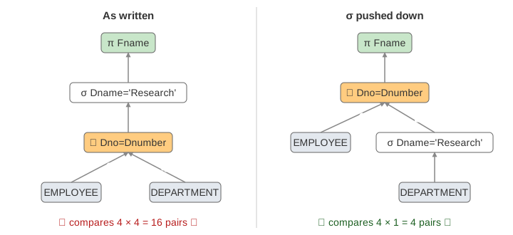
The condition Dname = 'Research' only reads DEPARTMENT columns, so σ can run before the join. The tree changes, the answer does not, and the join compares 4 pairs instead of 16 (Demo: Q1 with σ pushed down). Rules like this one (push σ down, push π down, swap the inputs of ⋈, reorder joins) are the equivalence rules a query optimizer uses to pick a cheap tree. The SQL stays the same; only the plan changes.
See also How a SELECT Runs for the logical order of the SQL clauses, Nested Loop vs Hash Join vs Merge Join for faster ways to compute ⋈ than testing every pair, and MariaDB Rewrites a Query Tree for a real optimizer pushing conditions down.
What the page leaves out
Rename (ρ), division (÷, "employees who work on all projects") and the extended operators: aggregation and grouping (γ, SQL's GROUP BY), outer joins and outer union are only named. The page evaluates σ and ⋈ by testing rows one at a time; a real engine uses indexes, hash tables or sorting, and pipelines rows from one operator to the next instead of building each table in full. It also keeps set semantics everywhere, while SQL works on bags unless told DISTINCT. Relational calculus, the declarative twin of the algebra, is not shown.
See where this page fits on the Databases & Storage mind map.