The idea: tags you cannot see, words you can
A part-of-speech tagger labels every word of a sentence with its word class: noun, verb, preposition, determiner, … The same word can take different tags. In "time flies like an arrow", flies can be a verb or a plural noun, and like can be a verb or a preposition. A hidden Markov model (HMM) treats the tags as hidden states and the words as what they emit. The tagger counts the model's tables from a corpus that people have already tagged. Then it finds the most likely tag sequence for a new sentence with the Viterbi algorithm.
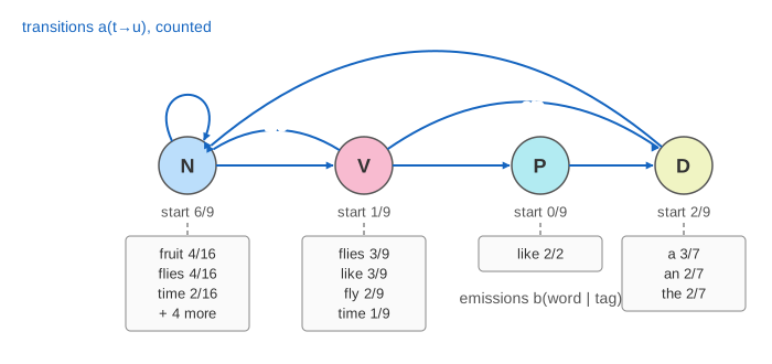
This page uses four tags: N noun, V verb, P preposition and D determiner. The corpus is 9 short sentences with 34 tagged words, such as fruit/N flies/N like/V a/D banana/N.
Counting the tables
The tables are not guessed. They are plain counts divided by row totals, which is the maximum likelihood estimate:
- Start π(t) = C(sentences that start with t) / C(sentences). Six of the 9 sentences start with a noun, so π(N) = 6/9.
- Transition a(t→u) = C(t followed by u) / C(t followed by any tag). A noun is followed by another tag 10 times: 8 times by a verb and 2 times by a noun. So a(N→V) = 8/10.
- Emission b(word | t) = C(word tagged t) / C(t). There are 9 verbs and 3 of them are flies, so b(flies | V) = 3/9. Every one of the 2 prepositions is like, so b(like | P) = 2/2.
Read b the right way round. It is the chance that a verb is the word flies, not the chance that flies is a verb. Most cells stay 0: in this corpus a noun is never followed by a determiner, and a determiner is always followed by a noun. Counting bigrams of words is the same idea, see N-gram Language Models; here the bigrams are pairs of tags. (Demo: count the corpus)
Scoring one tag sequence
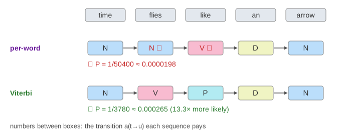
The HMM gives every tag sequence a probability together with the words. It is the start probability, then one transition and one emission per word. For time/N flies/V like/P an/D arrow/N:
π(N)·b(time|N)     6/9 × 2/16  = 1/12
× a(N→V)·b(flies|V)  8/10 × 3/9  → 1/45
× a(V→P)·b(like|P)   2/6 × 2/2   → 1/135
× a(P→D)·b(an|D)     2/2 × 2/7   → 2/945
× a(D→N)·b(arrow|N)  7/7 × 2/16  → 1/3780 ≈ 0.0002646
A 5-word sentence with 4 tags has 45 = 1024 tag sequences. With raw counts only 3 of them score above 0 here, because most transitions and emissions were never seen.
The trellis for a sentence
The tagger does not list the 1024 sequences. It fills a trellis: one column per word, one row per tag. Cell δi(t) is the probability of the best tag sequence for the first i words that ends with tag t. The first column is π(t)·b(word | t). Every later cell takes the best previous cell times the transition into t, then multiplies by b. The general recurrence, the forward algorithm and log-probabilities are on the Viterbi page. Here is what is special about tagging:
- Most cells are 0 for free. A tag that never emitted the word gets 0 without looking back: an is only ever D, so 3 of its 4 cells are 0.
- The ambiguous words keep two cells alive. At flies both N (0.004167) and V (0.02222) live. At like both V (0.001111, coming from flies/N) and P (0.007407, coming from flies/V) live.
- The next word settles it. At an the D cell compares V 0.001111 × 3/6 with P 0.007407 × 2/2 and keeps P.
(Demo: time flies like an arrow, word by word)
Back-pointers and traceback
Each live cell remembers which previous tag gave its best value: the back-pointer (blue arrow on the canvas). When the last column is full, the best sequence ends in its biggest cell: N for arrow, 0.0002646. Follow the back-pointers right to left: N ← D ← P ← V ← N. So the answer is time/N flies/V like/P an/D arrow/N, and its probability is exactly the 1/3780 worked out above.
Per-word tagging vs Viterbi
The simplest tagger ignores the context. It gives each word the tag it had most often in the corpus. time was N 2 times and V once, so it gets N. flies was N 4 times and V 3 times, so N. like was V 3 times and P 2 times, so V. For our sentence that gives N N V D N. The HMM gives this sequence P = 1/50400 ≈ 1.984·10−5, which is 13.3 times less likely than Viterbi's answer. The per-word tagger chose flies = N and like = V one word at a time. It never checked that N→N is rare (2/10), while V→P→D fits the words around them. (Demo: per-word tags vs Viterbi)
On real corpora the most-frequent-tag baseline is already about 92% accurate, because most words have only one tag. HMM taggers reach about 96–97% by getting the ambiguous words right from their neighbours.
One tag of memory
Now tag "fruit flies like a banana". The words after fruit are the same kind as before, and the model looks only one tag back. So Viterbi again picks N V P D N, with P = 1/2520 ≈ 0.0003968. That reads fruit as a noun that flies the way a banana does. A person reads "fruit flies" as insects that like bananas: N N V D N, which is exactly the per-word answer (P = 1/33600). The bigram HMM cannot see that fruit + flies make a compound. Real taggers use trigrams of tags and features of the words for this. (Demo: fruit flies like a banana)
| sentence | Viterbi | per-word | the reading people pick |
|---|---|---|---|
| time flies like an arrow | N V P D N ✓ | N N V D N | N V P D N |
| fruit flies like a banana | N V P D N | N N V D N ✓ | N N V D N |
Unseen words
"time flies like a dart" fails completely. dart is not in the corpus, so b(dart | t) = 0 for every tag, the whole last column is 0, and every one of the 1024 sequences has probability 0. One unknown word is enough to break a tagger built on raw counts. Real taggers smooth the emission table (see add-one smoothing on N-gram Language Models). They also guess an unknown word's tag from its shape: a final -s, -ed or -ing, a capital letter, digits. (Demo: an unseen word (dart))
See also Markov Chains and Random Walks for the chain the tags follow, Naive Bayes for a classifier built from the same kind of counts, and CYK Parsing for the next step after tagging: building the sentence's parse tree.
What the page leaves out
Real tag sets (17 Universal POS tags, 45 Penn Treebank tags); trigram HMMs that look two tags back; an end-of-sentence tag; smoothing and unknown-word models; log-probabilities, which long sentences need to avoid underflow; learning the tables without a tagged corpus (Baum–Welch); and the discriminative taggers that replaced HMMs: maximum-entropy Markov models, conditional random fields and neural taggers.